Affine Transformations#


Original author	Ana Huamán
Compatibility	OpenCV >= 3.0

Goal#

In this tutorial you will learn how to:

Use the OpenCV function cv::warpAffine to implement simple remapping routines.
Use the OpenCV function cv::getRotationMatrix2D to obtain a \(2 \times 3\) rotation matrix

Theory#

What is an Affine Transformation?#

A transformation that can be expressed in the form of a matrix multiplication (linear transformation) followed by a vector addition (translation).
From the above, we can use an Affine Transformation to express:
1. Rotations (linear transformation)
2. Translations (vector addition)
3. Scale operations (linear transformation)
you can see that, in essence, an Affine Transformation represents a relation between two images.
The usual way to represent an Affine Transformation is by using a \(2 \times 3\) matrix.

\[\begin{split}A = \begin{bmatrix} a_{00} & a_{01} \\ a_{10} & a_{11} \end{bmatrix}_{2 \times 2} B = \begin{bmatrix} b_{00} \\ b_{10} \end{bmatrix}_{2 \times 1}\end{split}\]

\[\begin{split}M = \begin{bmatrix} A & B \end{bmatrix} = \begin{bmatrix} a_{00} & a_{01} & b_{00} \\ a_{10} & a_{11} & b_{10} \end{bmatrix}_{2 \times 3}\end{split}\]

Considering that we want to transform a 2D vector \(X = \begin{bmatrix}x \\ y\end{bmatrix}\) by using \(A\) and \(B\), we can do the same with:

\(T = A \cdot \begin{bmatrix}x \\ y\end{bmatrix} + B\) or \(T = M \cdot [x, y, 1]^{T}\)

\[\begin{split}T = \begin{bmatrix} a_{00}x + a_{01}y + b_{00} \\ a_{10}x + a_{11}y + b_{10} \end{bmatrix}\end{split}\]

How do we get an Affine Transformation?#

We mentioned that an Affine Transformation is basically a relation between two images. The information about this relation can come, roughly, in two ways:
1. We know both \(X\) and \(T\) and we also know that they are related. Then our task is to find \(M\)
2. We know \(M\) and \(X\). To obtain \(T\) we only need to apply \(T = M \cdot X\). Our information for \(M\) may be explicit (i.e. have the 2-by-3 matrix) or it can come as a geometric relation between points.
Let’s explain this in a better way (b). Since \(M\) relates 2 images, we can analyze the simplest case in which it relates three points in both images. Look at the figure below:

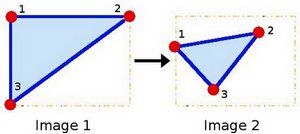
the points 1, 2 and 3 (forming a triangle in image 1) are mapped into image 2, still forming a triangle, but now they have changed notoriously. If we find the Affine Transformation with these 3 points (you can choose them as you like), then we can apply this found relation to all the pixels in an image.

Code#

What does this program do?
- Loads an image
- Applies an Affine Transform to the image. This transform is obtained from the relation between three points. We use the function cv::warpAffine for that purpose.
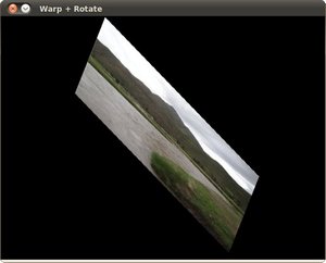
- Applies a Rotation to the image after being transformed. This rotation is with respect to the image center
- Waits until the user exits the program

C++

The tutorial’s code is shown below. You can also download it here

#include "opencv2/imgcodecs.hpp"
#include "opencv2/highgui.hpp"
#include "opencv2/geometry.hpp"
#include "opencv2/imgproc.hpp"
#include <iostream>

using namespace cv;
using namespace std;

int main( int argc, char** argv )
{
    CommandLineParser parser( argc, argv, "{@input | lena.jpg | input image}" );
    Mat src = imread( samples::findFile( parser.get<String>( "@input" ) ) );
    if( src.empty() )
    {
        cout << "Could not open or find the image!\n" << endl;
        cout << "Usage: " << argv[0] << " <Input image>" << endl;
        return -1;
    }

    Point2f srcTri[3];
    srcTri[0] = Point2f( 0.f, 0.f );
    srcTri[1] = Point2f( src.cols - 1.f, 0.f );
    srcTri[2] = Point2f( 0.f, src.rows - 1.f );

    Point2f dstTri[3];
    dstTri[0] = Point2f( 0.f, src.rows*0.33f );
    dstTri[1] = Point2f( src.cols*0.85f, src.rows*0.25f );
    dstTri[2] = Point2f( src.cols*0.15f, src.rows*0.7f );

    Mat warp_mat = getAffineTransform( srcTri, dstTri );

    /// Set the dst image the same type and size as src
    Mat warp_dst = Mat::zeros( src.rows, src.cols, src.type() );

    warpAffine( src, warp_dst, warp_mat, warp_dst.size() );

    Point center = Point( warp_dst.cols/2, warp_dst.rows/2 );
    double angle = -50.0;
    double scale = 0.6;

    Mat rot_mat = getRotationMatrix2D( center, angle, scale );

    Mat warp_rotate_dst;
    warpAffine( warp_dst, warp_rotate_dst, rot_mat, warp_dst.size() );

    imshow( "Source image", src );
    imshow( "Warp", warp_dst );
    imshow( "Warp + Rotate", warp_rotate_dst );

    waitKey();

    return 0;
}

Java

The tutorial’s code is shown below. You can also download it here

import org.opencv.core.Core;
import org.opencv.core.Mat;
import org.opencv.core.MatOfPoint2f;
import org.opencv.core.Point;
import org.opencv.highgui.HighGui;
import org.opencv.imgcodecs.Imgcodecs;
import org.opencv.imgproc.Imgproc;

class GeometricTransforms {
    public void run(String[] args) {
        String filename = args.length > 0 ? args[0] : "../data/lena.jpg";
        Mat src = Imgcodecs.imread(filename);
        if (src.empty()) {
            System.err.println("Cannot read image: " + filename);
            System.exit(0);
        }

        Point[] srcTri = new Point[3];
        srcTri[0] = new Point( 0, 0 );
        srcTri[1] = new Point( src.cols() - 1, 0 );
        srcTri[2] = new Point( 0, src.rows() - 1 );

        Point[] dstTri = new Point[3];
        dstTri[0] = new Point( 0, src.rows()*0.33 );
        dstTri[1] = new Point( src.cols()*0.85, src.rows()*0.25 );
        dstTri[2] = new Point( src.cols()*0.15, src.rows()*0.7 );

        Mat warpMat = Imgproc.getAffineTransform( new MatOfPoint2f(srcTri), new MatOfPoint2f(dstTri) );

        Mat warpDst = Mat.zeros( src.rows(), src.cols(), src.type() );

        Imgproc.warpAffine( src, warpDst, warpMat, warpDst.size() );

        Point center = new Point(warpDst.cols() / 2, warpDst.rows() / 2);
        double angle = -50.0;
        double scale = 0.6;

        Mat rotMat = Imgproc.getRotationMatrix2D( center, angle, scale );

        Mat warpRotateDst = new Mat();
        Imgproc.warpAffine( warpDst, warpRotateDst, rotMat, warpDst.size() );

        HighGui.imshow( "Source image", src );
        HighGui.imshow( "Warp", warpDst );
        HighGui.imshow( "Warp + Rotate", warpRotateDst );

        HighGui.waitKey(0);

        System.exit(0);
    }
}

public class GeometricTransformsDemo {
    public static void main(String[] args) {
        // Load the native OpenCV library
        System.loadLibrary(Core.NATIVE_LIBRARY_NAME);

        new GeometricTransforms().run(args);
    }
}

Python

The tutorial’s code is shown below. You can also download it here

from __future__ import print_function
import cv2 as cv
import numpy as np
import argparse

parser = argparse.ArgumentParser(description='Code for Affine Transformations tutorial.')
parser.add_argument('--input', help='Path to input image.', default='lena.jpg')
args = parser.parse_args()

src = cv.imread(cv.samples.findFile(args.input))
if src is None:
    print('Could not open or find the image:', args.input)
    exit(0)

srcTri = np.array( [[0, 0], [src.shape[1] - 1, 0], [0, src.shape[0] - 1]] ).astype(np.float32)
dstTri = np.array( [[0, src.shape[1]*0.33], [src.shape[1]*0.85, src.shape[0]*0.25], [src.shape[1]*0.15, src.shape[0]*0.7]] ).astype(np.float32)

warp_mat = cv.getAffineTransform(srcTri, dstTri)

warp_dst = cv.warpAffine(src, warp_mat, (src.shape[1], src.shape[0]))

# Rotating the image after Warp

center = (warp_dst.shape[1]//2, warp_dst.shape[0]//2)
angle = -50
scale = 0.6

rot_mat = cv.getRotationMatrix2D( center, angle, scale )

warp_rotate_dst = cv.warpAffine(warp_dst, rot_mat, (warp_dst.shape[1], warp_dst.shape[0]))

cv.imshow('Source image', src)
cv.imshow('Warp', warp_dst)
cv.imshow('Warp + Rotate', warp_rotate_dst)

cv.waitKey()

Result#

After compiling the code above, we can give it the path of an image as argument. For instance, for a picture like:

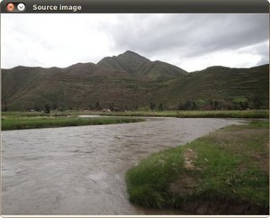
after applying the first Affine Transform we obtain:

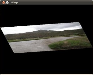
and finally, after applying a negative rotation (remember negative means clockwise) and a scale factor, we get:

Affine Transformations#

Goal#

Theory#

What is an Affine Transformation?#

How do we get an Affine Transformation?#

Code#

Explanation#

Result#