Histogram Calculation#


Original author	Ana Huamán
Compatibility	OpenCV >= 3.0

Goal#

In this tutorial you will learn how to:

Use the OpenCV function cv::split to divide an image into its correspondent planes.
To calculate histograms of arrays of images by using the OpenCV function cv::calcHist
To normalize an array by using the function cv::normalize

Note

In the last tutorial (Histogram Equalization) we talked about a particular kind of histogram called Image histogram. Now we will considerate it in its more general concept. Read on!

What are histograms?#

Histograms are collected counts of data organized into a set of predefined bins
When we say data we are not restricting it to be intensity values (as we saw in the previous Tutorial Histogram Equalization). The data collected can be whatever feature you find useful to describe your image.
Let’s see an example. Imagine that a Matrix contains information of an image (i.e. intensity in the range \(0-255\)):
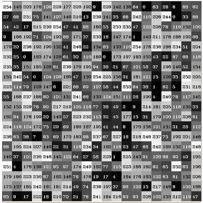
What happens if we want to count this data in an organized way? Since we know that the range of information value for this case is 256 values, we can segment our range in subparts (called bins) like:

\[\begin{split}\begin{array}{l} [0, 255] = { [0, 15] \cup [16, 31] \cup ....\cup [240,255] } \\ range = { bin_{1} \cup bin_{2} \cup ....\cup bin_{n = 15} } \end{array}\end{split}\]

and we can keep count of the number of pixels that fall in the range of each \(bin_{i}\). Applying this to the example above we get the image below ( axis x represents the bins and axis y the number of pixels in each of them).
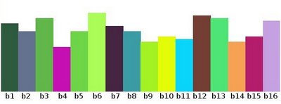
This was just a simple example of how an histogram works and why it is useful. An histogram can keep count not only of color intensities, but of whatever image features that we want to measure (i.e. gradients, directions, etc).
Let’s identify some parts of the histogram:
1. dims: The number of parameters you want to collect data of. In our example, dims = 1 because we are only counting the intensity values of each pixel (in a greyscale image).
2. bins: It is the number of subdivisions in each dim. In our example, bins = 16
3. range: The limits for the values to be measured. In this case: range = [0,255]
What if you want to count two features? In this case your resulting histogram would be a 3D plot (in which x and y would be \(bin_{x}\) and \(bin_{y}\) for each feature and z would be the number of counts for each combination of \((bin_{x}, bin_{y})\). The same would apply for more features (of course it gets trickier).

What OpenCV offers you#

For simple purposes, OpenCV implements the function cv::calcHist , which calculates the histogram of a set of arrays (usually images or image planes). It can operate with up to 32 dimensions. We will see it in the code below!

Code#

What does this program do?
- Loads an image
- Splits the image into its R, G and B planes using the function cv::split
- Calculate the Histogram of each 1-channel plane by calling the function cv::calcHist
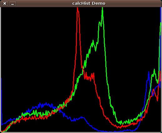
- Plot the three histograms in a window

C++

Downloadable code: Click here

Code at glance:

#include "opencv2/highgui.hpp"
#include "opencv2/imgcodecs.hpp"
#include "opencv2/imgproc.hpp"
#include <iostream>

using namespace std;
using namespace cv;

int main(int argc, char** argv)
{
    CommandLineParser parser( argc, argv, "{@input | lena.jpg | input image}" );
    Mat src = imread( samples::findFile( parser.get<String>( "@input" ) ), IMREAD_COLOR );
    if( src.empty() )
    {
        return EXIT_FAILURE;
    }

    //! [Separate the image in 3 places ( B, G and R )]
    vector<Mat> bgr_planes;
    split( src, bgr_planes );
    //! [Separate the image in 3 places ( B, G and R )]

    int histSize = 256;

    //! [Set the ranges ( for B,G,R) )]
    float range[] = { 0, 256 }; //the upper boundary is exclusive
    const float* histRange[] = { range };
    //! [Set the ranges ( for B,G,R) )]

    bool uniform = true, accumulate = false;

    Mat b_hist, g_hist, r_hist;
    calcHist( &bgr_planes[0], 1, 0, Mat(), b_hist, 1, &histSize, histRange, uniform, accumulate );
    calcHist( &bgr_planes[1], 1, 0, Mat(), g_hist, 1, &histSize, histRange, uniform, accumulate );
    calcHist( &bgr_planes[2], 1, 0, Mat(), r_hist, 1, &histSize, histRange, uniform, accumulate );

    //! [Draw the histograms for B, G and R]
    int hist_w = 512, hist_h = 400;
    int bin_w = cvRound( (double) hist_w/histSize );

    Mat histImage( hist_h, hist_w, CV_8UC3, Scalar( 0,0,0) );
    //! [Draw the histograms for B, G and R]

    //! [Normalize the result to ( 0, histImage.rows )]
    normalize(b_hist, b_hist, 0, histImage.rows, NORM_MINMAX, -1, Mat() );
    normalize(g_hist, g_hist, 0, histImage.rows, NORM_MINMAX, -1, Mat() );
    normalize(r_hist, r_hist, 0, histImage.rows, NORM_MINMAX, -1, Mat() );
    //! [Normalize the result to ( 0, histImage.rows )]

    for( int i = 1; i < histSize; i++ )
    {
        line( histImage, Point( bin_w*(i-1), hist_h - cvRound(b_hist.at<float>(i-1)) ),
              Point( bin_w*(i), hist_h - cvRound(b_hist.at<float>(i)) ),
              Scalar( 255, 0, 0), 2, 8, 0  );
        line( histImage, Point( bin_w*(i-1), hist_h - cvRound(g_hist.at<float>(i-1)) ),
              Point( bin_w*(i), hist_h - cvRound(g_hist.at<float>(i)) ),
              Scalar( 0, 255, 0), 2, 8, 0  );
        line( histImage, Point( bin_w*(i-1), hist_h - cvRound(r_hist.at<float>(i-1)) ),
              Point( bin_w*(i), hist_h - cvRound(r_hist.at<float>(i)) ),
              Scalar( 0, 0, 255), 2, 8, 0  );
    }

    imshow("Source image", src );
    imshow("calcHist Demo", histImage );
    waitKey();

    return EXIT_SUCCESS;
}

Java

Downloadable code: Click here

Code at glance:

import java.util.ArrayList;
import java.util.List;

import org.opencv.core.Core;
import org.opencv.core.CvType;
import org.opencv.core.Mat;
import org.opencv.core.MatOfFloat;
import org.opencv.core.MatOfInt;
import org.opencv.core.Point;
import org.opencv.core.Scalar;
import org.opencv.highgui.HighGui;
import org.opencv.imgcodecs.Imgcodecs;
import org.opencv.imgproc.Imgproc;

class CalcHist {
    public void run(String[] args) {
        String filename = args.length > 0 ? args[0] : "../data/lena.jpg";
        Mat src = Imgcodecs.imread(filename);
        if (src.empty()) {
            System.err.println("Cannot read image: " + filename);
            System.exit(0);
        }

        //! [Separate the image in 3 places ( B, G and R )]
        List<Mat> bgrPlanes = new ArrayList<>();
        Core.split(src, bgrPlanes);
        //! [Separate the image in 3 places ( B, G and R )]

        int histSize = 256;

        //! [Set the ranges ( for B,G,R) )]
        float[] range = {0, 256}; //the upper boundary is exclusive
        MatOfFloat histRange = new MatOfFloat(range);
        //! [Set the ranges ( for B,G,R) )]

        boolean accumulate = false;

        Mat bHist = new Mat(), gHist = new Mat(), rHist = new Mat();
        Imgproc.calcHist(bgrPlanes, new MatOfInt(0), new Mat(), bHist, new MatOfInt(histSize), histRange, accumulate);
        Imgproc.calcHist(bgrPlanes, new MatOfInt(1), new Mat(), gHist, new MatOfInt(histSize), histRange, accumulate);
        Imgproc.calcHist(bgrPlanes, new MatOfInt(2), new Mat(), rHist, new MatOfInt(histSize), histRange, accumulate);

        //! [Draw the histograms for B, G and R]
        int histW = 512, histH = 400;
        int binW = (int) Math.round((double) histW / histSize);

        Mat histImage = new Mat( histH, histW, CvType.CV_8UC3, new Scalar( 0,0,0) );
        //! [Draw the histograms for B, G and R]

        //! [Normalize the result to ( 0, histImage.rows )]
        Core.normalize(bHist, bHist, 0, histImage.rows(), Core.NORM_MINMAX);
        Core.normalize(gHist, gHist, 0, histImage.rows(), Core.NORM_MINMAX);
        Core.normalize(rHist, rHist, 0, histImage.rows(), Core.NORM_MINMAX);
        //! [Normalize the result to ( 0, histImage.rows )]

        float[] bHistData = new float[(int) (bHist.total() * bHist.channels())];
        bHist.get(0, 0, bHistData);
        float[] gHistData = new float[(int) (gHist.total() * gHist.channels())];
        gHist.get(0, 0, gHistData);
        float[] rHistData = new float[(int) (rHist.total() * rHist.channels())];
        rHist.get(0, 0, rHistData);

        for( int i = 1; i < histSize; i++ ) {
            Imgproc.line(histImage, new Point(binW * (i - 1), histH - Math.round(bHistData[i - 1])),
                    new Point(binW * (i), histH - Math.round(bHistData[i])), new Scalar(255, 0, 0), 2);
            Imgproc.line(histImage, new Point(binW * (i - 1), histH - Math.round(gHistData[i - 1])),
                    new Point(binW * (i), histH - Math.round(gHistData[i])), new Scalar(0, 255, 0), 2);
            Imgproc.line(histImage, new Point(binW * (i - 1), histH - Math.round(rHistData[i - 1])),
                    new Point(binW * (i), histH - Math.round(rHistData[i])), new Scalar(0, 0, 255), 2);
        }

        HighGui.imshow( "Source image", src );
        HighGui.imshow( "calcHist Demo", histImage );
        HighGui.waitKey(0);

        System.exit(0);
    }
}

public class CalcHistDemo {
    public static void main(String[] args) {
        // Load the native OpenCV library
        System.loadLibrary(Core.NATIVE_LIBRARY_NAME);

        new CalcHist().run(args);
    }
}

Python

Downloadable code: Click here

Code at glance:

from __future__ import print_function
from __future__ import division
import cv2 as cv
import numpy as np
import argparse

parser = argparse.ArgumentParser(description='Code for Histogram Calculation tutorial.')
parser.add_argument('--input', help='Path to input image.', default='lena.jpg')
args = parser.parse_args()

src = cv.imread(cv.samples.findFile(args.input))
if src is None:
    print('Could not open or find the image:', args.input)
    exit(0)

## [Separate the image in 3 places ( B, G and R )]
bgr_planes = cv.split(src)
## [Separate the image in 3 places ( B, G and R )]

histSize = 256

## [Set the ranges ( for B,G,R) )]
histRange = (0, 256) # the upper boundary is exclusive
## [Set the ranges ( for B,G,R) )]

accumulate = False

b_hist = cv.calcHist(bgr_planes, [0], None, [histSize], histRange, accumulate=accumulate)
g_hist = cv.calcHist(bgr_planes, [1], None, [histSize], histRange, accumulate=accumulate)
r_hist = cv.calcHist(bgr_planes, [2], None, [histSize], histRange, accumulate=accumulate)

## [Draw the histograms for B, G and R]
hist_w = 512
hist_h = 400
bin_w = int(round( hist_w/histSize ))

histImage = np.zeros((hist_h, hist_w, 3), dtype=np.uint8)
## [Draw the histograms for B, G and R]

## [Normalize the result to ( 0, histImage.rows )]
cv.normalize(b_hist, b_hist, alpha=0, beta=hist_h, norm_type=cv.NORM_MINMAX)
cv.normalize(g_hist, g_hist, alpha=0, beta=hist_h, norm_type=cv.NORM_MINMAX)
cv.normalize(r_hist, r_hist, alpha=0, beta=hist_h, norm_type=cv.NORM_MINMAX)
## [Normalize the result to ( 0, histImage.rows )]

for i in range(1, histSize):
    cv.line(histImage, ( bin_w*(i-1), hist_h - int(b_hist[i-1]) ),
            ( bin_w*(i), hist_h - int(b_hist[i]) ),
            ( 255, 0, 0), thickness=2)
    cv.line(histImage, ( bin_w*(i-1), hist_h - int(g_hist[i-1]) ),
            ( bin_w*(i), hist_h - int(g_hist[i]) ),
            ( 0, 255, 0), thickness=2)
    cv.line(histImage, ( bin_w*(i-1), hist_h - int(r_hist[i-1]) ),
            ( bin_w*(i), hist_h - int(r_hist[i]) ),
            ( 0, 0, 255), thickness=2)

cv.imshow('Source image', src)
cv.imshow('calcHist Demo', histImage)
cv.waitKey()

Result#

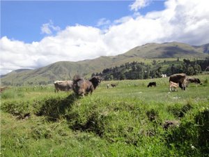
Using as input argument an image like the one shown below:
Produces the following histogram:

Histogram Calculation#

Goal#

What are histograms?#

What OpenCV offers you#

Code#

Explanation#

Result#