 |
OpenCV 4.14.0-pre
Open Source Computer Vision
|
 |
OpenCV 4.14.0-pre
Open Source Computer Vision
|
Prev Tutorial: Adding borders to your images
Next Tutorial: Laplace Operator
| Original author | Ana Huamán |
| Compatibility | OpenCV >= 3.0 |
In this tutorial you will learn how to:

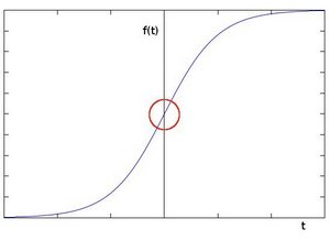
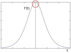
You can easily notice that in an edge, the pixel intensity changes in a notorious way. A good way to express changes is by using derivatives. A high change in gradient indicates a major change in the image.


Assuming that the image to be operated is \(I\):
We calculate two derivatives:
\[G_{x} = \begin{bmatrix} -1 & 0 & +1 \\ -2 & 0 & +2 \\ -1 & 0 & +1 \end{bmatrix} * I\]
\[G_{y} = \begin{bmatrix} -1 & -2 & -1 \\ 0 & 0 & 0 \\ +1 & +2 & +1 \end{bmatrix} * I\]
At each point of the image we calculate an approximation of the gradient in that point by combining both results above:
\[G = \sqrt{ G_{x}^{2} + G_{y}^{2} }\]
Although sometimes the following simpler equation is used:
\[G = |G_{x}| + |G_{y}|\]
3, the Sobel kernel shown above may produce noticeable inaccuracies (after all, Sobel is only an approximation of the derivative). OpenCV addresses this inaccuracy for kernels of size 3 by using the Scharr() function. This is as fast but more accurate than the standard Sobel function. It implements the following kernels: \[G_{x} = \begin{bmatrix} -3 & 0 & +3 \\ -10 & 0 & +10 \\ -3 & 0 & +3 \end{bmatrix}\]
\[G_{y} = \begin{bmatrix} -3 & -10 & -3 \\ 0 & 0 & 0 \\ +3 & +10 & +3 \end{bmatrix}\]
We calculate the "derivatives" in x and y directions. For this, we use the function Sobel() as shown below: The function takes the following arguments:
Notice that to calculate the gradient in x direction we use: \(x_{order}= 1\) and \(y_{order} = 0\). We do analogously for the y direction.
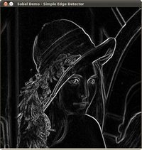
We try to approximate the gradient by adding both directional gradients (note that this is not an exact calculation at all! but it is good for our purposes).
