
Introduction to Principal Component Analysis (PCA)#
Goal#
In this tutorial you will learn how to:
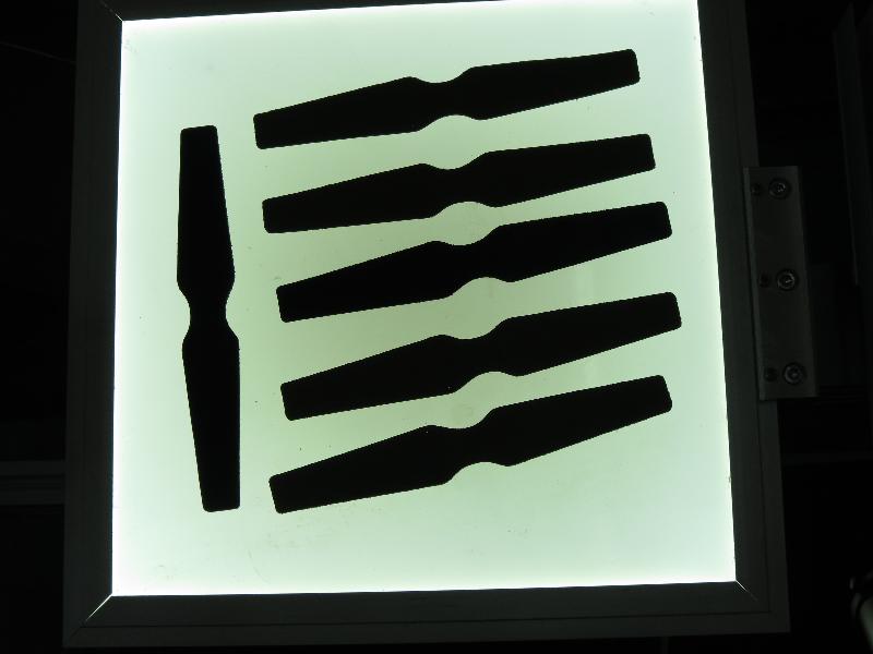
Use the OpenCV class [cv::PCA](#cv::PCA) to calculate the orientation of an object.
What is PCA?#
Principal Component Analysis (PCA) is a statistical procedure that extracts the most important features of a dataset.
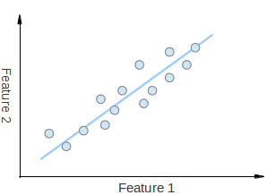
Consider that you have a set of 2D points as it is shown in the figure above. Each dimension corresponds to a feature you are interested in. Here some could argue that the points are set in a random order. However, if you have a better look you will see that there is a linear pattern (indicated by the blue line) which is hard to dismiss. A key point of PCA is the Dimensionality Reduction. Dimensionality Reduction is the process of reducing the number of the dimensions of the given dataset. For example, in the above case it is possible to approximate the set of points to a single line and therefore, reduce the dimensionality of the given points from 2D to 1D.
Moreover, you could also see that the points vary the most along the blue line, more than they vary along the Feature 1 or Feature 2 axes. This means that if you know the position of a point along the blue line you have more information about the point than if you only knew where it was on Feature 1 axis or Feature 2 axis.
Hence, PCA allows us to find the direction along which our data varies the most. In fact, the result of running PCA on the set of points in the diagram consist of 2 vectors called eigenvectors which are the principal components of the data set.
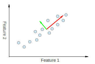
The size of each eigenvector is encoded in the corresponding eigenvalue and indicates how much the data vary along the principal component. The beginning of the eigenvectors is the center of all points in the data set. Applying PCA to N-dimensional data set yields N N-dimensional eigenvectors, N eigenvalues and 1 N-dimensional center point. Enough theory, let’s see how we can put these ideas into code.
How are the eigenvectors and eigenvalues computed?#
The goal is to transform a given data set X of dimension p to an alternative data set Y of smaller dimension L. Equivalently, we are seeking to find the matrix Y, where Y is the Karhunen–Loève transform (KLT) of matrix X:
Organize the data set
Suppose you have data comprising a set of observations of p variables, and you want to reduce the data so that each observation can be described with only L variables, L < p. Suppose further, that the data are arranged as a set of n data vectors \( x_1...x_n \) with each \( x_i \) representing a single grouped observation of the p variables.
Write \( x_1...x_n \) as row vectors, each of which has p columns.
Place the row vectors into a single matrix X of dimensions \( n\times p \).
Calculate the empirical mean
Find the empirical mean along each dimension \( j = 1, ..., p \).
Place the calculated mean values into an empirical mean vector u of dimensions \( p\times 1 \).
\[ \mathbf{u[j]} = \frac{1}{n}\sum_{i=1}^{n}\mathbf{X[i,j]} \]
Calculate the deviations from the mean
Mean subtraction is an integral part of the solution towards finding a principal component basis that minimizes the mean square error of approximating the data. Hence, we proceed by centering the data as follows:
Subtract the empirical mean vector u from each row of the data matrix X.
Store mean-subtracted data in the \( n\times p \) matrix B.
\[ \mathbf{B} = \mathbf{X} - \mathbf{h}\mathbf{u^{T}} \]where h is an \( n\times 1 \) column vector of all 1s:
\[ h[i] = 1, i = 1, ..., n \]
Find the covariance matrix
Find the \( p\times p \) empirical covariance matrix C from the outer product of matrix B with itself:
\[ \mathbf{C} = \frac{1}{n-1} \mathbf{B^{*}} \cdot \mathbf{B} \]where * is the conjugate transpose operator. Note that if B consists entirely of real numbers, which is the case in many applications, the “conjugate transpose” is the same as the regular transpose.
Find the eigenvectors and eigenvalues of the covariance matrix
Compute the matrix V of eigenvectors which diagonalizes the covariance matrix C:
\[ \mathbf{V^{-1}} \mathbf{C} \mathbf{V} = \mathbf{D} \]where D is the diagonal matrix of eigenvalues of C.
Matrix D will take the form of an \( p \times p \) diagonal matrix:
\[\begin{split}D[k,l] = \left\{\begin{matrix} \lambda_k, k = l \\ 0, k \neq l \end{matrix}\right.\end{split}\]here, \( \lambda_j \) is the j-th eigenvalue of the covariance matrix C
Matrix V, also of dimension p x p, contains p column vectors, each of length p, which represent the p eigenvectors of the covariance matrix C.
The eigenvalues and eigenvectors are ordered and paired. The j th eigenvalue corresponds to the j th eigenvector.
Source Code#
Downloadable code: Click here
Code at glance:
#include "opencv2/core.hpp"
#include "opencv2/imgproc.hpp"
#include "opencv2/geometry.hpp"
#include "opencv2/highgui.hpp"
#include <iostream>

using namespace std;
using namespace cv;

// Function declarations
void drawAxis(Mat&, Point, Point, Scalar, const float);
double getOrientation(const vector<Point> &, Mat&);

void drawAxis(Mat& img, Point p, Point q, Scalar colour, const float scale = 0.2)
{
    double angle = atan2( (double) p.y - q.y, (double) p.x - q.x ); // angle in radians
    double hypotenuse = sqrt( (double) (p.y - q.y) * (p.y - q.y) + (p.x - q.x) * (p.x - q.x));

    // Here we lengthen the arrow by a factor of scale
    q.x = (int) (p.x - scale * hypotenuse * cos(angle));
    q.y = (int) (p.y - scale * hypotenuse * sin(angle));
    line(img, p, q, colour, 1, LINE_AA);

    // create the arrow hooks
    p.x = (int) (q.x + 9 * cos(angle + CV_PI / 4));
    p.y = (int) (q.y + 9 * sin(angle + CV_PI / 4));
    line(img, p, q, colour, 1, LINE_AA);

    p.x = (int) (q.x + 9 * cos(angle - CV_PI / 4));
    p.y = (int) (q.y + 9 * sin(angle - CV_PI / 4));
    line(img, p, q, colour, 1, LINE_AA);
}

double getOrientation(const vector<Point> &pts, Mat &img)
{
    //Construct a buffer used by the pca analysis
    int sz = static_cast<int>(pts.size());
    Mat data_pts = Mat(sz, 2, CV_64F);
    for (int i = 0; i < data_pts.rows; i++)
    {
        data_pts.at<double>(i, 0) = pts[i].x;
        data_pts.at<double>(i, 1) = pts[i].y;
    }

    //Perform PCA analysis
    PCA pca_analysis(data_pts, Mat(), PCA::DATA_AS_ROW);

    //Store the center of the object
    Point cntr = Point(static_cast<int>(pca_analysis.mean.at<double>(0, 0)),
                      static_cast<int>(pca_analysis.mean.at<double>(0, 1)));

    //Store the eigenvalues and eigenvectors
    vector<Point2d> eigen_vecs(2);
    vector<double> eigen_val(2);
    for (int i = 0; i < 2; i++)
    {
        eigen_vecs[i] = Point2d(pca_analysis.eigenvectors.at<double>(i, 0),
                                pca_analysis.eigenvectors.at<double>(i, 1));

        eigen_val[i] = pca_analysis.eigenvalues.at<double>(i);
    }

    // Draw the principal components
    circle(img, cntr, 3, Scalar(255, 0, 255), 2);
    Point p1 = cntr + 0.02 * Point(static_cast<int>(eigen_vecs[0].x * eigen_val[0]), static_cast<int>(eigen_vecs[0].y * eigen_val[0]));
    Point p2 = cntr - 0.02 * Point(static_cast<int>(eigen_vecs[1].x * eigen_val[1]), static_cast<int>(eigen_vecs[1].y * eigen_val[1]));
    drawAxis(img, cntr, p1, Scalar(0, 255, 0), 1);
    drawAxis(img, cntr, p2, Scalar(255, 255, 0), 5);

    double angle = atan2(eigen_vecs[0].y, eigen_vecs[0].x); // orientation in radians

    return angle;
}

int main(int argc, char** argv)
{
    // Load image
    CommandLineParser parser(argc, argv, "{@input | pca_test1.jpg | input image}");
    parser.about( "This program demonstrates how to use OpenCV PCA to extract the orientation of an object.\n" );
    parser.printMessage();

    Mat src = imread( samples::findFile( parser.get<String>("@input") ) );

    // Check if image is loaded successfully
    if(src.empty())
    {
        cout << "Problem loading image!!!" << endl;
        return EXIT_FAILURE;
    }

    imshow("src", src);

    // Convert image to grayscale
    Mat gray;
    cvtColor(src, gray, COLOR_BGR2GRAY);

    // Convert image to binary
    Mat bw;
    threshold(gray, bw, 50, 255, THRESH_BINARY | THRESH_OTSU);

    // Find all the contours in the thresholded image
    vector<vector<Point> > contours;
    findContours(bw, contours, RETR_LIST, CHAIN_APPROX_NONE);

    for (size_t i = 0; i < contours.size(); i++)
    {
        // Calculate the area of each contour
        double area = contourArea(contours[i]);
        // Ignore contours that are too small or too large
        if (area < 1e2 || 1e5 < area) continue;

        // Draw each contour only for visualisation purposes
        drawContours(src, contours, static_cast<int>(i), Scalar(0, 0, 255), 2);
        // Find the orientation of each shape
        getOrientation(contours[i], src);
    }

    imshow("output", src);

    waitKey();
    return EXIT_SUCCESS;
}
Downloadable code: Click here
Code at glance:
import java.util.ArrayList;
import java.util.List;

import org.opencv.core.Core;
import org.opencv.core.CvType;
import org.opencv.core.Mat;
import org.opencv.core.MatOfPoint;
import org.opencv.core.Point;
import org.opencv.core.Scalar;
import org.opencv.highgui.HighGui;
import org.opencv.imgcodecs.Imgcodecs;
import org.opencv.imgproc.Imgproc;

//This program demonstrates how to use OpenCV PCA to extract the orientation of an object.
class IntroductionToPCA {
    private void drawAxis(Mat img, Point p_, Point q_, Scalar colour, float scale) {
        Point p = new Point(p_.x, p_.y);
        Point q = new Point(q_.x, q_.y);
        double angle = Math.atan2(p.y - q.y, p.x - q.x); // angle in radians
        double hypotenuse = Math.sqrt((p.y - q.y) * (p.y - q.y) + (p.x - q.x) * (p.x - q.x));

        // Here we lengthen the arrow by a factor of scale
        q.x = (int) (p.x - scale * hypotenuse * Math.cos(angle));
        q.y = (int) (p.y - scale * hypotenuse * Math.sin(angle));
        Imgproc.line(img, p, q, colour, 1, Imgproc.LINE_AA, 0);

        // create the arrow hooks
        p.x = (int) (q.x + 9 * Math.cos(angle + Math.PI / 4));
        p.y = (int) (q.y + 9 * Math.sin(angle + Math.PI / 4));
        Imgproc.line(img, p, q, colour, 1, Imgproc.LINE_AA, 0);

        p.x = (int) (q.x + 9 * Math.cos(angle - Math.PI / 4));
        p.y = (int) (q.y + 9 * Math.sin(angle - Math.PI / 4));
        Imgproc.line(img, p, q, colour, 1, Imgproc.LINE_AA, 0);
    }

    private double getOrientation(MatOfPoint ptsMat, Mat img) {
        List<Point> pts = ptsMat.toList();
        // Construct a buffer used by the pca analysis
        int sz = pts.size();
        Mat dataPts = new Mat(sz, 2, CvType.CV_64F);
        double[] dataPtsData = new double[(int) (dataPts.total() * dataPts.channels())];
        for (int i = 0; i < dataPts.rows(); i++) {
            dataPtsData[i * dataPts.cols()] = pts.get(i).x;
            dataPtsData[i * dataPts.cols() + 1] = pts.get(i).y;
        }
        dataPts.put(0, 0, dataPtsData);

        // Perform PCA analysis
        Mat mean = new Mat();
        Mat eigenvectors = new Mat();
        Mat eigenvalues = new Mat();
        Core.PCACompute2(dataPts, mean, eigenvectors, eigenvalues);
        double[] meanData = new double[(int) (mean.total() * mean.channels())];
        mean.get(0, 0, meanData);

        // Store the center of the object
        Point cntr = new Point(meanData[0], meanData[1]);

        // Store the eigenvalues and eigenvectors
        double[] eigenvectorsData = new double[(int) (eigenvectors.total() * eigenvectors.channels())];
        double[] eigenvaluesData = new double[(int) (eigenvalues.total() * eigenvalues.channels())];
        eigenvectors.get(0, 0, eigenvectorsData);
        eigenvalues.get(0, 0, eigenvaluesData);

        // Draw the principal components
        Imgproc.circle(img, cntr, 3, new Scalar(255, 0, 255), 2);
        Point p1 = new Point(cntr.x + 0.02 * eigenvectorsData[0] * eigenvaluesData[0],
                cntr.y + 0.02 * eigenvectorsData[1] * eigenvaluesData[0]);
        Point p2 = new Point(cntr.x - 0.02 * eigenvectorsData[2] * eigenvaluesData[1],
                cntr.y - 0.02 * eigenvectorsData[3] * eigenvaluesData[1]);
        drawAxis(img, cntr, p1, new Scalar(0, 255, 0), 1);
        drawAxis(img, cntr, p2, new Scalar(255, 255, 0), 5);

        double angle = Math.atan2(eigenvectorsData[1], eigenvectorsData[0]); // orientation in radians

        return angle;
    }

    public void run(String[] args) {
        // Load image
        String filename = args.length > 0 ? args[0] : "../data/pca_test1.jpg";
        Mat src = Imgcodecs.imread(filename);

        // Check if image is loaded successfully
        if (src.empty()) {
            System.err.println("Cannot read image: " + filename);
            System.exit(0);
        }

        Mat srcOriginal = src.clone();
        HighGui.imshow("src", srcOriginal);

        // Convert image to grayscale
        Mat gray = new Mat();
        Imgproc.cvtColor(src, gray, Imgproc.COLOR_BGR2GRAY);

        // Convert image to binary
        Mat bw = new Mat();
        Imgproc.threshold(gray, bw, 50, 255, Imgproc.THRESH_BINARY | Imgproc.THRESH_OTSU);

        // Find all the contours in the thresholded image
        List<MatOfPoint> contours = new ArrayList<>();
        Mat hierarchy = new Mat();
        Imgproc.findContours(bw, contours, hierarchy, Imgproc.RETR_LIST, Imgproc.CHAIN_APPROX_NONE);

        for (int i = 0; i < contours.size(); i++) {
            // Calculate the area of each contour
            double area = Imgproc.contourArea(contours.get(i));
            // Ignore contours that are too small or too large
            if (area < 1e2 || 1e5 < area)
                continue;

            // Draw each contour only for visualisation purposes
            Imgproc.drawContours(src, contours, i, new Scalar(0, 0, 255), 2);
            // Find the orientation of each shape
            getOrientation(contours.get(i), src);
        }

        HighGui.imshow("output", src);

        HighGui.waitKey();
        System.exit(0);
    }
}

public class IntroductionToPCADemo {
    public static void main(String[] args) {
        // Load the native OpenCV library
        System.loadLibrary(Core.NATIVE_LIBRARY_NAME);

        new IntroductionToPCA().run(args);
    }
}
Downloadable code: Click here
Code at glance:
from __future__ import print_function
from __future__ import division
import cv2 as cv
import numpy as np
import argparse
from math import atan2, cos, sin, sqrt, pi

def drawAxis(img, p_, q_, colour, scale):
    p = list(p_)
    q = list(q_)
    angle = atan2(p[1] - q[1], p[0] - q[0]) # angle in radians
    hypotenuse = sqrt((p[1] - q[1]) * (p[1] - q[1]) + (p[0] - q[0]) * (p[0] - q[0]))

    # Here we lengthen the arrow by a factor of scale
    q[0] = p[0] - scale * hypotenuse * cos(angle)
    q[1] = p[1] - scale * hypotenuse * sin(angle)
    cv.line(img, (int(p[0]), int(p[1])), (int(q[0]), int(q[1])), colour, 1, cv.LINE_AA)

    # create the arrow hooks
    p[0] = q[0] + 9 * cos(angle + pi / 4)
    p[1] = q[1] + 9 * sin(angle + pi / 4)
    cv.line(img, (int(p[0]), int(p[1])), (int(q[0]), int(q[1])), colour, 1, cv.LINE_AA)

    p[0] = q[0] + 9 * cos(angle - pi / 4)
    p[1] = q[1] + 9 * sin(angle - pi / 4)
    cv.line(img, (int(p[0]), int(p[1])), (int(q[0]), int(q[1])), colour, 1, cv.LINE_AA)

def getOrientation(pts, img):
    # Construct a buffer used by the pca analysis
    sz = len(pts)
    data_pts = np.empty((sz, 2), dtype=np.float64)
    for i in range(data_pts.shape[0]):
        data_pts[i,0] = pts[i,0,0]
        data_pts[i,1] = pts[i,0,1]

    # Perform PCA analysis
    mean = np.empty((0))
    mean, eigenvectors, eigenvalues = cv.PCACompute2(data_pts, mean)

    # Store the center of the object
    cntr = (int(mean[0,0]), int(mean[0,1]))

    # Draw the principal components
    cv.circle(img, cntr, 3, (255, 0, 255), 2)
    p1 = (cntr[0] + 0.02 * eigenvectors[0,0] * eigenvalues[0,0], cntr[1] + 0.02 * eigenvectors[0,1] * eigenvalues[0,0])
    p2 = (cntr[0] - 0.02 * eigenvectors[1,0] * eigenvalues[1,0], cntr[1] - 0.02 * eigenvectors[1,1] * eigenvalues[1,0])
    drawAxis(img, cntr, p1, (0, 255, 0), 1)
    drawAxis(img, cntr, p2, (255, 255, 0), 5)

    angle = atan2(eigenvectors[0,1], eigenvectors[0,0]) # orientation in radians

    return angle

# Load image
parser = argparse.ArgumentParser(description='Code for Introduction to Principal Component Analysis (PCA) tutorial.\
                                              This program demonstrates how to use OpenCV PCA to extract the orientation of an object.')
parser.add_argument('--input', help='Path to input image.', default='pca_test1.jpg')
args = parser.parse_args()

src = cv.imread(cv.samples.findFile(args.input))
# Check if image is loaded successfully
if src is None:
    print('Could not open or find the image: ', args.input)
    exit(0)

cv.imshow('src', src)

# Convert image to grayscale
gray = cv.cvtColor(src, cv.COLOR_BGR2GRAY)

# Convert image to binary
_, bw = cv.threshold(gray, 50, 255, cv.THRESH_BINARY | cv.THRESH_OTSU)

# Find all the contours in the thresholded image
contours, _ = cv.findContours(bw, cv.RETR_LIST, cv.CHAIN_APPROX_NONE)

for i, c in enumerate(contours):
    # Calculate the area of each contour
    area = cv.contourArea(c)
    # Ignore contours that are too small or too large
    if area < 1e2 or 1e5 < area:
        continue

    # Draw each contour only for visualisation purposes
    cv.drawContours(src, contours, i, (0, 0, 255), 2)
    # Find the orientation of each shape
    getOrientation(c, src)

cv.imshow('output', src)
cv.waitKey()
Note
Another example using PCA for dimensionality reduction while maintaining an amount of variance can be found at [opencv_source_code/samples/cpp/pca.cpp](https://github.com/opencv/opencv/tree/5.x/samples/cpp/pca.cpp)
Explanation#
Read image and convert it to binary
Here we apply the necessary pre-processing procedures in order to be able to detect the objects of interest.
// Load image
CommandLineParser parser(argc, argv, "{@input | pca_test1.jpg | input image}");
parser.about( "This program demonstrates how to use OpenCV PCA to extract the orientation of an object.\n" );
parser.printMessage();

Mat src = imread( samples::findFile( parser.get<String>("@input") ) );

// Check if image is loaded successfully
if(src.empty())
{
    cout << "Problem loading image!!!" << endl;
    return EXIT_FAILURE;
}

imshow("src", src);

// Convert image to grayscale
Mat gray;
cvtColor(src, gray, COLOR_BGR2GRAY);

// Convert image to binary
Mat bw;
threshold(gray, bw, 50, 255, THRESH_BINARY | THRESH_OTSU);
// Load image
String filename = args.length > 0 ? args[0] : "../data/pca_test1.jpg";
Mat src = Imgcodecs.imread(filename);

// Check if image is loaded successfully
if (src.empty()) {
    System.err.println("Cannot read image: " + filename);
    System.exit(0);
}

Mat srcOriginal = src.clone();
HighGui.imshow("src", srcOriginal);

// Convert image to grayscale
Mat gray = new Mat();
Imgproc.cvtColor(src, gray, Imgproc.COLOR_BGR2GRAY);

// Convert image to binary
Mat bw = new Mat();
Imgproc.threshold(gray, bw, 50, 255, Imgproc.THRESH_BINARY | Imgproc.THRESH_OTSU);
# Load image
parser = argparse.ArgumentParser(description='Code for Introduction to Principal Component Analysis (PCA) tutorial.\
                                              This program demonstrates how to use OpenCV PCA to extract the orientation of an object.')
parser.add_argument('--input', help='Path to input image.', default='pca_test1.jpg')
args = parser.parse_args()

src = cv.imread(cv.samples.findFile(args.input))
# Check if image is loaded successfully
if src is None:
    print('Could not open or find the image: ', args.input)
    exit(0)

cv.imshow('src', src)

# Convert image to grayscale
gray = cv.cvtColor(src, cv.COLOR_BGR2GRAY)

# Convert image to binary
_, bw = cv.threshold(gray, 50, 255, cv.THRESH_BINARY | cv.THRESH_OTSU)
Extract objects of interest
Then find and filter contours by size and obtain the orientation of the remaining ones.
// Find all the contours in the thresholded image
vector<vector<Point> > contours;
findContours(bw, contours, RETR_LIST, CHAIN_APPROX_NONE);

for (size_t i = 0; i < contours.size(); i++)
{
    // Calculate the area of each contour
    double area = contourArea(contours[i]);
    // Ignore contours that are too small or too large
    if (area < 1e2 || 1e5 < area) continue;

    // Draw each contour only for visualisation purposes
    drawContours(src, contours, static_cast<int>(i), Scalar(0, 0, 255), 2);
    // Find the orientation of each shape
    getOrientation(contours[i], src);
}
// Find all the contours in the thresholded image
List<MatOfPoint> contours = new ArrayList<>();
Mat hierarchy = new Mat();
Imgproc.findContours(bw, contours, hierarchy, Imgproc.RETR_LIST, Imgproc.CHAIN_APPROX_NONE);

for (int i = 0; i < contours.size(); i++) {
    // Calculate the area of each contour
    double area = Imgproc.contourArea(contours.get(i));
    // Ignore contours that are too small or too large
    if (area < 1e2 || 1e5 < area)
        continue;

    // Draw each contour only for visualisation purposes
    Imgproc.drawContours(src, contours, i, new Scalar(0, 0, 255), 2);
    // Find the orientation of each shape
    getOrientation(contours.get(i), src);
}
# Find all the contours in the thresholded image
contours, _ = cv.findContours(bw, cv.RETR_LIST, cv.CHAIN_APPROX_NONE)

for i, c in enumerate(contours):
    # Calculate the area of each contour
    area = cv.contourArea(c)
    # Ignore contours that are too small or too large
    if area < 1e2 or 1e5 < area:
        continue

    # Draw each contour only for visualisation purposes
    cv.drawContours(src, contours, i, (0, 0, 255), 2)
    # Find the orientation of each shape
    getOrientation(c, src)
Extract orientation
Orientation is extracted by the call of getOrientation() function, which performs all the PCA procedure.
//Construct a buffer used by the pca analysis
int sz = static_cast<int>(pts.size());
Mat data_pts = Mat(sz, 2, CV_64F);
for (int i = 0; i < data_pts.rows; i++)
{
    data_pts.at<double>(i, 0) = pts[i].x;
    data_pts.at<double>(i, 1) = pts[i].y;
}

//Perform PCA analysis
PCA pca_analysis(data_pts, Mat(), PCA::DATA_AS_ROW);

//Store the center of the object
Point cntr = Point(static_cast<int>(pca_analysis.mean.at<double>(0, 0)),
                  static_cast<int>(pca_analysis.mean.at<double>(0, 1)));

//Store the eigenvalues and eigenvectors
vector<Point2d> eigen_vecs(2);
vector<double> eigen_val(2);
for (int i = 0; i < 2; i++)
{
    eigen_vecs[i] = Point2d(pca_analysis.eigenvectors.at<double>(i, 0),
                            pca_analysis.eigenvectors.at<double>(i, 1));

    eigen_val[i] = pca_analysis.eigenvalues.at<double>(i);
}
// Construct a buffer used by the pca analysis
int sz = pts.size();
Mat dataPts = new Mat(sz, 2, CvType.CV_64F);
double[] dataPtsData = new double[(int) (dataPts.total() * dataPts.channels())];
for (int i = 0; i < dataPts.rows(); i++) {
    dataPtsData[i * dataPts.cols()] = pts.get(i).x;
    dataPtsData[i * dataPts.cols() + 1] = pts.get(i).y;
}
dataPts.put(0, 0, dataPtsData);

// Perform PCA analysis
Mat mean = new Mat();
Mat eigenvectors = new Mat();
Mat eigenvalues = new Mat();
Core.PCACompute2(dataPts, mean, eigenvectors, eigenvalues);
double[] meanData = new double[(int) (mean.total() * mean.channels())];
mean.get(0, 0, meanData);

// Store the center of the object
Point cntr = new Point(meanData[0], meanData[1]);

// Store the eigenvalues and eigenvectors
double[] eigenvectorsData = new double[(int) (eigenvectors.total() * eigenvectors.channels())];
double[] eigenvaluesData = new double[(int) (eigenvalues.total() * eigenvalues.channels())];
eigenvectors.get(0, 0, eigenvectorsData);
eigenvalues.get(0, 0, eigenvaluesData);
# Construct a buffer used by the pca analysis
sz = len(pts)
data_pts = np.empty((sz, 2), dtype=np.float64)
for i in range(data_pts.shape[0]):
    data_pts[i,0] = pts[i,0,0]
    data_pts[i,1] = pts[i,0,1]

# Perform PCA analysis
mean = np.empty((0))
mean, eigenvectors, eigenvalues = cv.PCACompute2(data_pts, mean)

# Store the center of the object
cntr = (int(mean[0,0]), int(mean[0,1]))
First the data need to be arranged in a matrix with size n x 2, where n is the number of data points we have. Then we can perform that PCA analysis. The calculated mean (i.e. center of mass) is stored in the cntr variable and the eigenvectors and eigenvalues are stored in the corresponding std::vector’s.
Visualize result
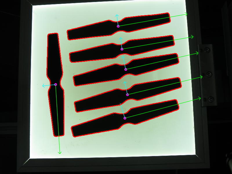
The final result is visualized through the drawAxis() function, where the principal components are drawn in lines, and each eigenvector is multiplied by its eigenvalue and translated to the mean position.
// Draw the principal components
circle(img, cntr, 3, Scalar(255, 0, 255), 2);
Point p1 = cntr + 0.02 * Point(static_cast<int>(eigen_vecs[0].x * eigen_val[0]), static_cast<int>(eigen_vecs[0].y * eigen_val[0]));
Point p2 = cntr - 0.02 * Point(static_cast<int>(eigen_vecs[1].x * eigen_val[1]), static_cast<int>(eigen_vecs[1].y * eigen_val[1]));
drawAxis(img, cntr, p1, Scalar(0, 255, 0), 1);
drawAxis(img, cntr, p2, Scalar(255, 255, 0), 5);

double angle = atan2(eigen_vecs[0].y, eigen_vecs[0].x); // orientation in radians
// Draw the principal components
Imgproc.circle(img, cntr, 3, new Scalar(255, 0, 255), 2);
Point p1 = new Point(cntr.x + 0.02 * eigenvectorsData[0] * eigenvaluesData[0],
        cntr.y + 0.02 * eigenvectorsData[1] * eigenvaluesData[0]);
Point p2 = new Point(cntr.x - 0.02 * eigenvectorsData[2] * eigenvaluesData[1],
        cntr.y - 0.02 * eigenvectorsData[3] * eigenvaluesData[1]);
drawAxis(img, cntr, p1, new Scalar(0, 255, 0), 1);
drawAxis(img, cntr, p2, new Scalar(255, 255, 0), 5);

double angle = Math.atan2(eigenvectorsData[1], eigenvectorsData[0]); // orientation in radians
# Draw the principal components
cv.circle(img, cntr, 3, (255, 0, 255), 2)
p1 = (cntr[0] + 0.02 * eigenvectors[0,0] * eigenvalues[0,0], cntr[1] + 0.02 * eigenvectors[0,1] * eigenvalues[0,0])
p2 = (cntr[0] - 0.02 * eigenvectors[1,0] * eigenvalues[1,0], cntr[1] - 0.02 * eigenvectors[1,1] * eigenvalues[1,0])
drawAxis(img, cntr, p1, (0, 255, 0), 1)
drawAxis(img, cntr, p2, (255, 255, 0), 5)

angle = atan2(eigenvectors[0,1], eigenvectors[0,0]) # orientation in radians
double angle = atan2( (double) p.y - q.y, (double) p.x - q.x ); // angle in radians
double hypotenuse = sqrt( (double) (p.y - q.y) * (p.y - q.y) + (p.x - q.x) * (p.x - q.x));

// Here we lengthen the arrow by a factor of scale
q.x = (int) (p.x - scale * hypotenuse * cos(angle));
q.y = (int) (p.y - scale * hypotenuse * sin(angle));
line(img, p, q, colour, 1, LINE_AA);

// create the arrow hooks
p.x = (int) (q.x + 9 * cos(angle + CV_PI / 4));
p.y = (int) (q.y + 9 * sin(angle + CV_PI / 4));
line(img, p, q, colour, 1, LINE_AA);

p.x = (int) (q.x + 9 * cos(angle - CV_PI / 4));
p.y = (int) (q.y + 9 * sin(angle - CV_PI / 4));
line(img, p, q, colour, 1, LINE_AA);
double angle = Math.atan2(p.y - q.y, p.x - q.x); // angle in radians
double hypotenuse = Math.sqrt((p.y - q.y) * (p.y - q.y) + (p.x - q.x) * (p.x - q.x));

// Here we lengthen the arrow by a factor of scale
q.x = (int) (p.x - scale * hypotenuse * Math.cos(angle));
q.y = (int) (p.y - scale * hypotenuse * Math.sin(angle));
Imgproc.line(img, p, q, colour, 1, Imgproc.LINE_AA, 0);

// create the arrow hooks
p.x = (int) (q.x + 9 * Math.cos(angle + Math.PI / 4));
p.y = (int) (q.y + 9 * Math.sin(angle + Math.PI / 4));
Imgproc.line(img, p, q, colour, 1, Imgproc.LINE_AA, 0);

p.x = (int) (q.x + 9 * Math.cos(angle - Math.PI / 4));
p.y = (int) (q.y + 9 * Math.sin(angle - Math.PI / 4));
Imgproc.line(img, p, q, colour, 1, Imgproc.LINE_AA, 0);
angle = atan2(p[1] - q[1], p[0] - q[0]) # angle in radians
hypotenuse = sqrt((p[1] - q[1]) * (p[1] - q[1]) + (p[0] - q[0]) * (p[0] - q[0]))

# Here we lengthen the arrow by a factor of scale
q[0] = p[0] - scale * hypotenuse * cos(angle)
q[1] = p[1] - scale * hypotenuse * sin(angle)
cv.line(img, (int(p[0]), int(p[1])), (int(q[0]), int(q[1])), colour, 1, cv.LINE_AA)

# create the arrow hooks
p[0] = q[0] + 9 * cos(angle + pi / 4)
p[1] = q[1] + 9 * sin(angle + pi / 4)
cv.line(img, (int(p[0]), int(p[1])), (int(q[0]), int(q[1])), colour, 1, cv.LINE_AA)

p[0] = q[0] + 9 * cos(angle - pi / 4)
p[1] = q[1] + 9 * sin(angle - pi / 4)
cv.line(img, (int(p[0]), int(p[1])), (int(q[0]), int(q[1])), colour, 1, cv.LINE_AA)
Results#
The code opens an image, finds the orientation of the detected objects of interest and then visualizes the result by drawing the contours of the detected objects of interest, the center point, and the x-axis, y-axis regarding the extracted orientation.