Contour Features#

Goal#

To find the different features of contours, like area, perimeter, centroid, bounding box etc
You will learn plenty of functions related to contours.

1. Moments#

Image moments help you to calculate some features like center of mass of the object, area of the object etc. Check out the wikipedia page on Image Moments

We use the function: cv.moments (array, binaryImage = false)

Parameters

array: raster image (single-channel, 8-bit or floating-point 2D array) or an array ( 1×N or N×1 ) of 2D points.
binaryImage: if it is true, all non-zero image pixels are treated as 1’s. The parameter is used for images only.

Try it#

From this moments, you can extract useful data like area, centroid etc. Centroid is given by the relations, \(C_x = \frac{M_{10}}{M_{00}}\) and \(C_y = \frac{M_{01}}{M_{00}}\). This can be done as follows:

let cx = M.m10/M.m00
let cy = M.m01/M.m00

2. Contour Area#

Contour area is given by the function cv.contourArea() or from moments, M[‘m00’].

We use the function: cv.contourArea (contour, oriented = false)

Parameters

contour: input vector of 2D points (contour vertices)
oriented: oriented area flag. If it is true, the function returns a signed area value, depending on the contour orientation (clockwise or counter-clockwise). Using this feature you can determine orientation of a contour by taking the sign of an area. By default, the parameter is false, which means that the absolute value is returned.

Try it#

3. Contour Perimeter#

It is also called arc length. It can be found out using cv.arcLength() function.

We use the function: cv.arcLength (curve, closed)

Parameters

curve: input vector of 2D points.
closed: flag indicating whether the curve is closed or not.

Try it#

4. Contour Approximation#

It approximates a contour shape to another shape with less number of vertices depending upon the precision we specify. It is an implementation of Douglas-Peucker algorithm. Check the wikipedia page for algorithm and demonstration.

We use the function: cv.approxPolyDP (curve, approxCurve, epsilon, closed)

Parameters

curve: input vector of 2D points stored in cv.Mat.
approxCurve: result of the approximation. The type should match the type of the input curve.
epsilon: parameter specifying the approximation accuracy. This is the maximum distance between the original curve and its approximation.
closed: If true, the approximated curve is closed (its first and last vertices are connected). Otherwise, it is not closed.

Try it#

5. Convex Hull#

Convex Hull will look similar to contour approximation, but it is not (Both may provide same results in some cases). Here, cv.convexHull() function checks a curve for convexity defects and corrects it. Generally speaking, convex curves are the curves which are always bulged out, or at-least flat. And if it is bulged inside, it is called convexity defects. For example, check the below image of hand. Red line shows the convex hull of hand. The double-sided arrow marks shows the convexity defects, which are the local maximum deviations of hull from contours.

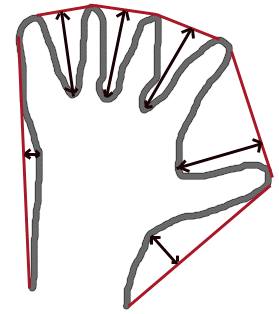
We use the function: cv.convexHull (points, hull, clockwise = false, returnPoints = true)

Parameters

points: input 2D point set.
hull: output convex hull.
clockwise: orientation flag. If it is true, the output convex hull is oriented clockwise. Otherwise, it is oriented counter-clockwise. The assumed coordinate system has its X axis pointing to the right, and its Y axis pointing upwards.
returnPoints: operation flag. In case of a matrix, when the flag is true, the function returns convex hull points. Otherwise, it returns indices of the convex hull points.

Try it#

6. Checking Convexity#

There is a function to check if a curve is convex or not, cv.isContourConvex(). It just return whether True or False. Not a big deal.

cv.isContourConvex(cnt);

7. Bounding Rectangle#

There are two types of bounding rectangles.

7.a. Straight Bounding Rectangle#

It is a straight rectangle, it doesn’t consider the rotation of the object. So area of the bounding rectangle won’t be minimum.

We use the function: cv.boundingRect (points)

Parameters

points: input 2D point set.

Try it#

7.b. Rotated Rectangle#

Here, bounding rectangle is drawn with minimum area, so it considers the rotation also.

We use the function: cv.minAreaRect (points)

Parameters

points: input 2D point set.

Try it#

8. Minimum Enclosing Circle#

Next we find the circumcircle of an object using the function cv.minEnclosingCircle(). It is a circle which completely covers the object with minimum area.

We use the functions: cv.minEnclosingCircle (points)

Parameters

points: input 2D point set.

cv.circle (img, center, radius, color, thickness = 1, lineType = cv.LINE_8, shift = 0)

Parameters

img: image where the circle is drawn.
center: center of the circle.
radius: radius of the circle.
color: circle color.
thickness: thickness of the circle outline, if positive. Negative thickness means that a filled circle is to be drawn.
lineType: type of the circle boundary.
shift: number of fractional bits in the coordinates of the center and in the radius value.

Try it#

9. Fitting an Ellipse#

Next one is to fit an ellipse to an object. It returns the rotated rectangle in which the ellipse is inscribed. We use the functions: cv.fitEllipse (points)

Parameters

points: input 2D point set.

cv.ellipse1 (img, box, color, thickness = 1, lineType = cv.LINE_8)

Parameters

img: image.
box: alternative ellipse representation via RotatedRect. This means that the function draws an ellipse inscribed in the rotated rectangle.
color: ellipse color.
thickness: thickness of the ellipse arc outline, if positive. Otherwise, this indicates that a filled ellipse sector is to be drawn.
lineType: type of the ellipse boundary.

Try it#

10. Fitting a Line#

Similarly we can fit a line to a set of points. We can approximate a straight line to it.

We use the functions: cv.fitLine (points, line, distType, param, reps, aeps)

Parameters

points: input 2D point set.
line: output line parameters. It should be a Mat of 4 elements[vx, vy, x0, y0], where [vx, vy] is a normalized vector collinear to the line and [x0, y0] is a point on the line.
distType: distance used by the M-estimator(see cv.DistanceTypes).
param: numerical parameter ( C ) for some types of distances. If it is 0, an optimal value is chosen.
reps: sufficient accuracy for the radius (distance between the coordinate origin and the line).
aeps: sufficient accuracy for the angle. 0.01 would be a good default value for reps and aeps.

cv.line (img, pt1, pt2, color, thickness = 1, lineType = cv.LINE_8, shift = 0)

Parameters

img: image.
pt1: first point of the line segment.
pt2: second point of the line segment.
color: line color.
thickness: line thickness.
lineType: type of the line,.
shift: number of fractional bits in the point coordinates.