Prev Tutorial: Adding (blending) two images using OpenCV
Next Tutorial: Discrete Fourier Transform
| |
| Original author | Ana Huamán |
| Compatibility | OpenCV >= 3.0 |
Goal
In this tutorial you will learn how to:
- Access pixel values
- Initialize a matrix with zeros
- Learn what cv::saturate_cast does and why it is useful
- Get some cool info about pixel transformations
- Improve the brightness of an image on a practical example
Theory
- Note
- The explanation below belongs to the book Computer Vision: Algorithms and Applications by Richard Szeliski
Image Processing
- A general image processing operator is a function that takes one or more input images and produces an output image.
- Image transforms can be seen as:
- Point operators (pixel transforms)
- Neighborhood (area-based) operators
Pixel Transforms
- In this kind of image processing transform, each output pixel's value depends on only the corresponding input pixel value (plus, potentially, some globally collected information or parameters).
- Examples of such operators include brightness and contrast adjustments as well as color correction and transformations.
Brightness and contrast adjustments
Two commonly used point processes are multiplication and addition with a constant:
\[g(x) = \alpha f(x) + \beta\]
- The parameters \(\alpha > 0\) and \(\beta\) are often called the gain and bias parameters; sometimes these parameters are said to control contrast and brightness respectively.
You can think of \(f(x)\) as the source image pixels and \(g(x)\) as the output image pixels. Then, more conveniently we can write the expression as:
\[g(i,j) = \alpha \cdot f(i,j) + \beta\]
where \(i\) and \(j\) indicates that the pixel is located in the i-th row and j-th column.
Code
C++
- Downloadable code: Click here
- The following code performs the operation \(g(i,j) = \alpha \cdot f(i,j) + \beta\) :
#include <iostream>
using std::cin;
using std::cout;
using std::endl;
int main(
int argc,
char** argv )
{
Mat image = imread( samples::findFile( parser.get<
String>(
"@input" ) ) );
{
cout << "Could not open or find the image!\n" << endl;
cout << "Usage: " << argv[0] << " <Input image>" << endl;
return -1;
}
Mat new_image = Mat::zeros( image.
size(), image.
type() );
double alpha = 1.0;
int beta = 0;
cout << " Basic Linear Transforms " << endl;
cout << "-------------------------" << endl;
cout << "* Enter the alpha value [1.0-3.0]: "; cin >> alpha;
cout << "* Enter the beta value [0-100]: "; cin >> beta;
for(
int y = 0; y < image.
rows; y++ ) {
for(
int x = 0; x < image.
cols; x++ ) {
for(
int c = 0; c < image.
channels(); c++ ) {
saturate_cast<uchar>( alpha*image.
at<
Vec3b>(y,x)[c] + beta );
}
}
}
imshow(
"Original Image", image);
imshow(
"New Image", new_image);
return 0;
}
Designed for command line parsing.
Definition utility.hpp:890
n-dimensional dense array class
Definition mat.hpp:840
MatSize size
Definition mat.hpp:2226
_Tp & at(int i0=0)
Returns a reference to the specified array element.
int channels() const
Returns the number of matrix channels.
int cols
Definition mat.hpp:2204
bool empty() const
Returns true if the array has no elements.
int rows
the number of rows and columns or (-1, -1) when the matrix has more than 2 dimensions
Definition mat.hpp:2204
int type() const
Returns the type of a matrix element.
Template class for short numerical vectors, a partial case of Matx.
Definition matx.hpp:369
std::string String
Definition cvstd.hpp:151
void imshow(const String &winname, InputArray mat)
Displays an image in the specified window.
int waitKey(int delay=0)
Waits for a pressed key.
int main(int argc, char *argv[])
Definition highgui_qt.cpp:3
Java
- Downloadable code: Click here
- The following code performs the operation \(g(i,j) = \alpha \cdot f(i,j) + \beta\) :
import java.util.Scanner;
import org.opencv.core.Core;
import org.opencv.core.Mat;
import org.opencv.highgui.HighGui;
import org.opencv.imgcodecs.Imgcodecs;
class BasicLinearTransforms {
private byte saturate(double val) {
int iVal = (int) Math.round(val);
iVal = iVal > 255 ? 255 : (iVal < 0 ? 0 : iVal);
return (byte) iVal;
}
public void run(String[] args) {
String imagePath = args.length > 0 ? args[0] : "../data/lena.jpg";
Mat image = Imgcodecs.imread(imagePath);
if (image.empty()) {
System.out.println("Empty image: " + imagePath);
System.exit(0);
}
Mat newImage = Mat.zeros(image.size(), image.type());
double alpha = 1.0;
int beta = 0;
System.out.println(" Basic Linear Transforms ");
System.out.println("-------------------------");
try (Scanner scanner = new Scanner(System.in)) {
System.out.print("* Enter the alpha value [1.0-3.0]: ");
alpha = scanner.nextDouble();
System.out.print("* Enter the beta value [0-100]: ");
beta = scanner.nextInt();
}
byte[] imageData = new byte[(int) (image.total()*image.channels())];
image.get(0, 0, imageData);
byte[] newImageData = new byte[(int) (newImage.total()*newImage.channels())];
for (int y = 0; y < image.rows(); y++) {
for (int x = 0; x < image.cols(); x++) {
for (int c = 0; c < image.channels(); c++) {
double pixelValue = imageData[(y * image.cols() + x) * image.channels() + c];
pixelValue = pixelValue < 0 ? pixelValue + 256 : pixelValue;
newImageData[(y * image.cols() + x) * image.channels() + c]
= saturate(alpha * pixelValue + beta);
}
}
}
newImage.put(0, 0, newImageData);
HighGui.imshow("Original Image", image);
HighGui.imshow("New Image", newImage);
HighGui.waitKey();
System.exit(0);
}
}
public class BasicLinearTransformsDemo {
public static void main(String[] args) {
System.loadLibrary(Core.NATIVE_LIBRARY_NAME);
new BasicLinearTransforms().run(args);
}
}
Python
- Downloadable code: Click here
- The following code performs the operation \(g(i,j) = \alpha \cdot f(i,j) + \beta\) :
from __future__ import print_function
from builtins import input
import cv2 as cv
import numpy as np
import argparse
parser = argparse.ArgumentParser(description='Code for Changing the contrast and brightness of an image! tutorial.')
parser.add_argument('--input', help='Path to input image.', default='lena.jpg')
args = parser.parse_args()
if image is None:
print('Could not open or find the image: ', args.input)
exit(0)
new_image = np.zeros(image.shape, image.dtype)
alpha = 1.0
beta = 0
print(' Basic Linear Transforms ')
print('-------------------------')
try:
alpha = float(input('* Enter the alpha value [1.0-3.0]: '))
beta = int(input('* Enter the beta value [0-100]: '))
except ValueError:
print('Error, not a number')
for y in range(image.shape[0]):
for x in range(image.shape[1]):
for c in range(image.shape[2]):
new_image[y,x,c] = np.clip(alpha*image[y,x,c] + beta, 0, 255)
cv::String findFile(const cv::String &relative_path, bool required=true, bool silentMode=false)
Try to find requested data file.
Mat imread(const String &filename, int flags=IMREAD_COLOR_BGR)
Loads an image from a file.
Explanation
- We load an image using cv::imread and save it in a Mat object:
C++
{
cout << "Could not open or find the image!\n" << endl;
cout << "Usage: " << argv[0] << " <Input image>" << endl;
return -1;
}
Java
String imagePath = args.length > 0 ? args[0] :
"../data/lena.jpg";
Mat image = Imgcodecs.imread(imagePath);
if (image.empty()) {
System.out.println("Empty image: " + imagePath);
System.exit(0);
}
Python
parser = argparse.ArgumentParser(description='Code for Changing the contrast and brightness of an image! tutorial.')
parser.add_argument('--input', help='Path to input image.', default='lena.jpg')
args = parser.parse_args()
if image is None:
print('Could not open or find the image: ', args.input)
exit(0)
- Now, since we will make some transformations to this image, we need a new Mat object to store it. Also, we want this to have the following features:
- Initial pixel values equal to zero
- Same size and type as the original image
C++
Mat new_image = Mat::zeros( image.
size(), image.
type() );
Java
Mat newImage = Mat.zeros(image.size(), image.type());
Python
new_image = np.zeros(image.shape, image.dtype)
We observe that cv::Mat::zeros returns a Matlab-style zero initializer based on image.size() and image.type()
- We ask now the values of \(\alpha\) and \(\beta\) to be entered by the user:
C++
double alpha = 1.0;
int beta = 0;
cout << " Basic Linear Transforms " << endl;
cout << "-------------------------" << endl;
cout << "* Enter the alpha value [1.0-3.0]: "; cin >> alpha;
cout << "* Enter the beta value [0-100]: "; cin >> beta;
Java
double alpha = 1.0;
int beta = 0;
System.out.println(" Basic Linear Transforms ");
System.out.println("-------------------------");
try (Scanner scanner = new Scanner(System.in)) {
System.out.print("* Enter the alpha value [1.0-3.0]: ");
alpha = scanner.nextDouble();
System.out.print("* Enter the beta value [0-100]: ");
beta = scanner.nextInt();
}
Python
alpha = 1.0
beta = 0
print(' Basic Linear Transforms ')
print('-------------------------')
try:
alpha = float(input('* Enter the alpha value [1.0-3.0]: '))
beta = int(input('* Enter the beta value [0-100]: '))
except ValueError:
print('Error, not a number')
- Now, to perform the operation \(g(i,j) = \alpha \cdot f(i,j) + \beta\) we will access to each pixel in image. Since we are operating with BGR images, we will have three values per pixel (B, G and R), so we will also access them separately. Here is the piece of code:
C++
for(
int y = 0; y < image.
rows; y++ ) {
for(
int x = 0; x < image.
cols; x++ ) {
for(
int c = 0; c < image.
channels(); c++ ) {
saturate_cast<uchar>( alpha*image.
at<
Vec3b>(y,x)[c] + beta );
}
}
}
Java
byte[] imageData = new byte[(int) (image.total()*image.channels())];
image.get(0, 0, imageData);
byte[] newImageData = new byte[(int) (newImage.total()*newImage.channels())];
for (int y = 0; y < image.rows(); y++) {
for (int x = 0; x < image.cols(); x++) {
for (int c = 0; c < image.channels(); c++) {
double pixelValue = imageData[(y * image.cols() + x) * image.channels() + c];
pixelValue = pixelValue < 0 ? pixelValue + 256 : pixelValue;
newImageData[(y * image.cols() + x) * image.channels() + c]
= saturate(alpha * pixelValue + beta);
}
}
}
newImage.put(0, 0, newImageData);
Python
for y in range(image.shape[0]):
for x in range(image.shape[1]):
for c in range(image.shape[2]):
new_image[y,x,c] = np.clip(alpha*image[y,x,c] + beta, 0, 255)
Notice the following (C++ code only):
- To access each pixel in the images we are using this syntax: image.at<Vec3b>(y,x)[c] where y is the row, x is the column and c is B, G or R (0, 1 or 2).
- Since the operation \(\alpha \cdot p(i,j) + \beta\) can give values out of range or not integers (if \(\alpha\) is float), we use cv::saturate_cast to make sure the values are valid.
- Finally, we create windows and show the images, the usual way.
C++
imshow(
"Original Image", image);
imshow(
"New Image", new_image);
Java
HighGui.imshow("Original Image", image);
HighGui.imshow("New Image", newImage);
HighGui.waitKey();
Python
- Note
- Instead of using the for loops to access each pixel, we could have simply used this command:
C++
void convertTo(OutputArray m, int rtype, double alpha=1, double beta=0) const
Converts an array to another data type with optional scaling.
Java
image.convertTo(newImage, -1, alpha, beta);
Python
void convertScaleAbs(InputArray src, OutputArray dst, double alpha=1, double beta=0)
Scales, calculates absolute values, and converts the result to 8-bit.
where cv::Mat::convertTo would effectively perform *new_image = a*image + beta*. However, we wanted to show you how to access each pixel. In any case, both methods give the same result but convertTo is more optimized and works a lot faster.
Result
- Running our code and using \(\alpha = 2.2\) and \(\beta = 50\)
$ ./BasicLinearTransforms lena.jpg
Basic Linear Transforms
-------------------------
* Enter the alpha value [1.0-3.0]: 2.2
* Enter the beta value [0-100]: 50
- We get this:
Practical example
In this paragraph, we will put into practice what we have learned to correct an underexposed image by adjusting the brightness and the contrast of the image. We will also see another technique to correct the brightness of an image called gamma correction.
Brightness and contrast adjustments
Increasing (/ decreasing) the \(\beta\) value will add (/ subtract) a constant value to every pixel. Pixel values outside of the [0 ; 255] range will be saturated (i.e. a pixel value higher (/ lesser) than 255 (/ 0) will be clamped to 255 (/ 0)).
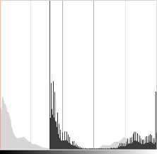
In light gray, histogram of the original image, in dark gray when brightness = 80 in Gimp
The histogram represents for each color level the number of pixels with that color level. A dark image will have many pixels with low color value and thus the histogram will present a peak in its left part. When adding a constant bias, the histogram is shifted to the right as we have added a constant bias to all the pixels.
The \(\alpha\) parameter will modify how the levels spread. If \( \alpha < 1 \), the color levels will be compressed and the result will be an image with less contrast.
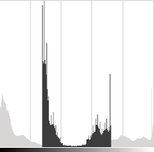
In light gray, histogram of the original image, in dark gray when contrast < 0 in Gimp
Note that these histograms have been obtained using the Brightness-Contrast tool in the Gimp software. The brightness tool should be identical to the \(\beta\) bias parameters but the contrast tool seems to differ to the \(\alpha\) gain where the output range seems to be centered with Gimp (as you can notice in the previous histogram).
It can occur that playing with the \(\beta\) bias will improve the brightness but in the same time the image will appear with a slight veil as the contrast will be reduced. The \(\alpha\) gain can be used to diminue this effect but due to the saturation, we will lose some details in the original bright regions.
Gamma correction
Gamma correction can be used to correct the brightness of an image by using a non linear transformation between the input values and the mapped output values:
\[O = \left( \frac{I}{255} \right)^{\gamma} \times 255\]
As this relation is non linear, the effect will not be the same for all the pixels and will depend to their original value.
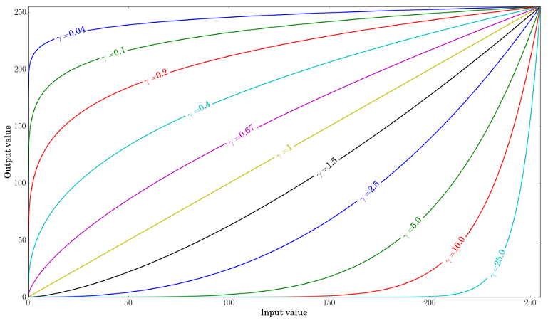
Plot for different values of gamma
When \( \gamma < 1 \), the original dark regions will be brighter and the histogram will be shifted to the right whereas it will be the opposite with \( \gamma > 1 \).
Correct an underexposed image
The following image has been corrected with: \( \alpha = 1.3 \) and \( \beta = 40 \).
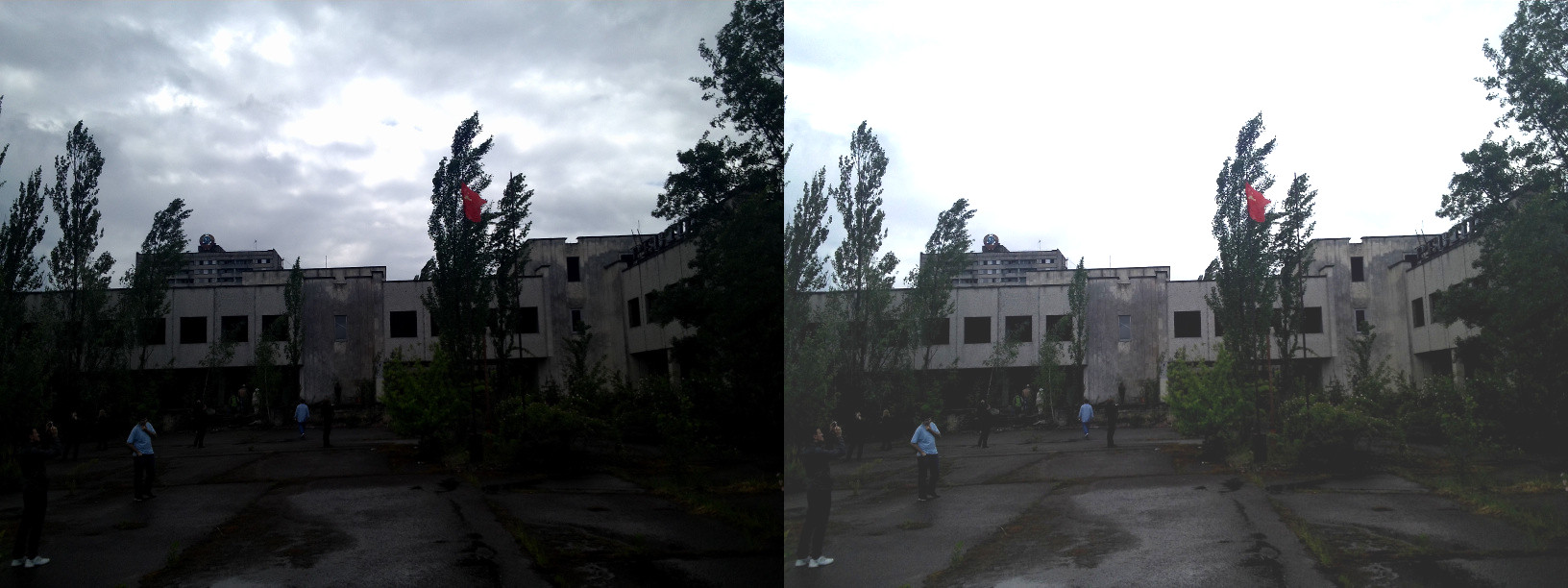
By Visem (Own work) [CC BY-SA 3.0], via Wikimedia Commons
The overall brightness has been improved but you can notice that the clouds are now greatly saturated due to the numerical saturation of the implementation used (highlight clipping in photography).
The following image has been corrected with: \( \gamma = 0.4 \).
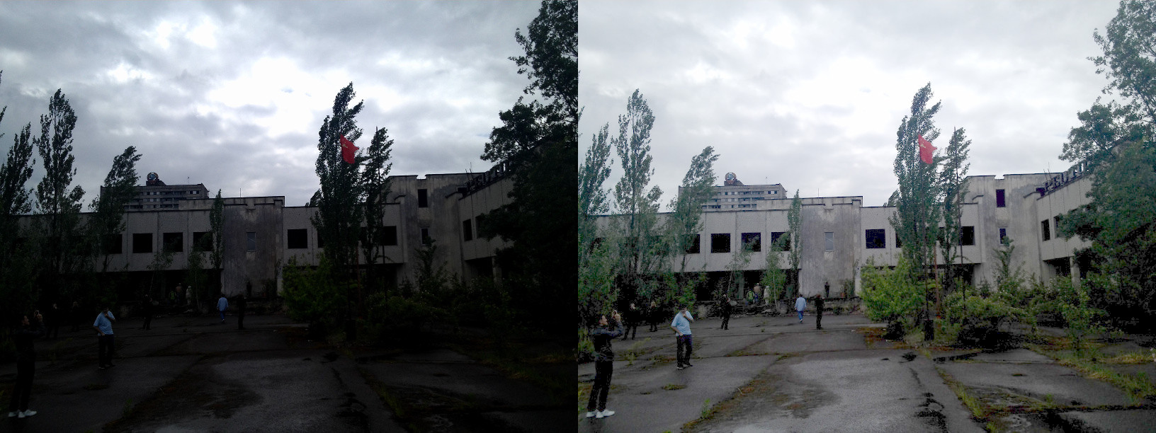
By Visem (Own work) [CC BY-SA 3.0], via Wikimedia Commons
The gamma correction should tend to add less saturation effect as the mapping is non linear and there is no numerical saturation possible as in the previous method.
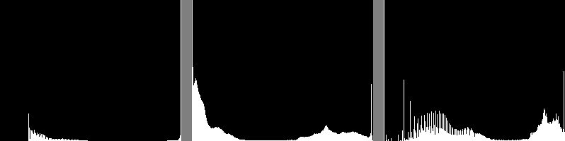
Left: histogram after alpha, beta correction ; Center: histogram of the original image ; Right: histogram after the gamma correction
The previous figure compares the histograms for the three images (the y-ranges are not the same between the three histograms). You can notice that most of the pixel values are in the lower part of the histogram for the original image. After \( \alpha \), \( \beta \) correction, we can observe a big peak at 255 due to the saturation as well as a shift in the right. After gamma correction, the histogram is shifted to the right but the pixels in the dark regions are more shifted (see the gamma curves figure) than those in the bright regions.
In this tutorial, you have seen two simple methods to adjust the contrast and the brightness of an image. They are basic techniques and are not intended to be used as a replacement of a raster graphics editor!
Code
C++
Code for the tutorial is here.
Java
Code for the tutorial is here.
Python
Code for the tutorial is here.
Code for the gamma correction:
C++
uchar* p = lookUpTable.ptr();
for( int i = 0; i < 256; ++i)
p[i] = saturate_cast<uchar>(pow(i / 255.0, gamma_) * 255.0);
LUT(img, lookUpTable, res);
Java
Mat lookUpTable = new Mat(1, 256, CvType.CV_8U);
byte[] lookUpTableData = new byte[(int) (lookUpTable.total()*lookUpTable.channels())];
for (int i = 0; i < lookUpTable.cols(); i++) {
lookUpTableData[i] = saturate(Math.pow(i / 255.0, gammaValue) * 255.0);
}
lookUpTable.put(0, 0, lookUpTableData);
Mat img = new Mat();
Core.LUT(matImgSrc, lookUpTable, img);
Python
lookUpTable = np.empty((1,256), np.uint8)
for i in range(256):
lookUpTable[0,i] = np.clip(pow(i / 255.0, gamma) * 255.0, 0, 255)
res =
cv.LUT(img_original, lookUpTable)
A look-up table is used to improve the performance of the computation as only 256 values needs to be calculated once.
Additional resources