Goal

In this chapter, we will understand the concepts of the k-Nearest Neighbour (kNN) algorithm.

Theory

kNN is one of the simplest classification algorithms available for supervised learning. The idea is to search for the closest match(es) of the test data in the feature space. We will look into it with the below image.

image

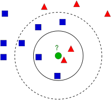
In the image, there are two families: Blue Squares and Red Triangles. We refer to each family as a Class. Their houses are shown in their town map which we call the Feature Space. You can consider a feature space as a space where all data are projected. For example, consider a 2D coordinate space. Each datum has two features, a x coordinate and a y coordinate. You can represent this datum in your 2D coordinate space, right? Now imagine that there are three features, you will need 3D space. Now consider N features: you need N-dimensional space, right? This N-dimensional space is its feature space. In our image, you can consider it as a 2D case with two features.

Now consider what happens if a new member comes into the town and creates a new home, which is shown as the green circle. He should be added to one of these Blue or Red families (or classes). We call that process, Classification. How exactly should this new member be classified? Since we are dealing with kNN, let us apply the algorithm.

One simple method is to check who is his nearest neighbour. From the image, it is clear that it is a member of the Red Triangle family. So he is classified as a Red Triangle. This method is called simply Nearest Neighbour classification, because classification depends only on the nearest neighbour.

But there is a problem with this approach! Red Triangle may be the nearest neighbour, but what if there are also a lot of Blue Squares nearby? Then Blue Squares have more strength in that locality than Red Triangles, so just checking the nearest one is not sufficient. Instead we may want to check some k nearest families. Then whichever family is the majority amongst them, the new guy should belong to that family. In our image, let's take k=3, i.e. consider the 3 nearest neighbours. The new member has two Red neighbours and one Blue neighbour (there are two Blues equidistant, but since k=3, we can take only one of them), so again he should be added to Red family. But what if we take k=7? Then he has 5 Blue neighbours and 2 Red neighbours and should be added to the Blue family. The result will vary with the selected value of k. Note that if k is not an odd number, we can get a tie, as would happen in the above case with k=4. We would see that our new member has 2 Red and 2 Blue neighbours as his four nearest neighbours and we would need to choose a method for breaking the tie to perform classification. So to reiterate, this method is called k-Nearest Neighbour since classification depends on the k nearest neighbours.

Again, in kNN, it is true we are considering k neighbours, but we are giving equal importance to all, right? Is this justified? For example, take the tied case of k=4. As we can see, the 2 Red neighbours are actually closer to the new member than the other 2 Blue neighbours, so he is more eligible to be added to the Red family. How do we mathematically explain that? We give some weights to each neighbour depending on their distance to the new-comer: those who are nearer to him get higher weights, while those that are farther away get lower weights. Then we add the total weights of each family separately and classify the new-comer as part of whichever family received higher total weights. This is called modified kNN or weighted kNN.

So what are some important things you see here?

Because we have to check the distance from the new-comer to all the existing houses to find the nearest neighbour(s), you need to have information about all of the houses in town, right? If there are plenty of houses and families, it takes a lot of memory, and also more time for calculation.
There is almost zero time for any kind of "training" or preparation. Our "learning" involves only memorizing (storing) the data, before testing and classifying.

Now let's see this algorithm at work in OpenCV.

kNN in OpenCV

We will do a simple example here, with two families (classes), just like above. Then in the next chapter, we will do an even better example.

So here, we label the Red family as Class-0 (so denoted by 0) and Blue family as Class-1 (denoted by 1). We create 25 neighbours or 25 training data, and label each of them as either part of Class-0 or Class-1. We can do this with the help of a Random Number Generator from NumPy.

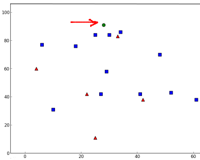
Then we can plot it with the help of Matplotlib. Red neighbours are shown as Red Triangles and Blue neighbours are shown as Blue Squares.

import cv2 as cv
import numpy as np
import matplotlib.pyplot as plt
 
# Feature set containing (x,y) values of 25 known/training data
trainData = np.random.randint(0,100,(25,2)).astype(np.float32)
 
# Label each one either Red or Blue with numbers 0 and 1
responses = np.random.randint(0,2,(25,1)).astype(np.float32)
 
# Take Red neighbours and plot them
red = trainData[responses.ravel()==0]
plt.scatter(red[:,0],red[:,1],80,'r','^')
 
# Take Blue neighbours and plot them
blue = trainData[responses.ravel()==1]
plt.scatter(blue[:,0],blue[:,1],80,'b','s')
 
plt.show()

You will get something similar to our first image. Since you are using a random number generator, you will get different data each time you run the code.

Next initiate the kNN algorithm and pass the trainData and responses to train the kNN. (Underneath the hood, it constructs a search tree: see the Additional Resources section below for more information on this.)

Then we will bring one new-comer and classify him as belonging to a family with the help of kNN in OpenCV. Before running kNN, we need to know something about our test data (data of new comers). Our data should be a floating point array with size \(number \; of \; testdata \times number \; of \; features\). Then we find the nearest neighbours of the new-comer. We can specify k: how many neighbours we want. (Here we used 3.) It returns:

The label given to the new-comer depending upon the kNN theory we saw earlier. If you want the Nearest Neighbour algorithm, just specify k=1.
The labels of the k-Nearest Neighbours.
The corresponding distances from the new-comer to each nearest neighbour.

So let's see how it works. The new-comer is marked in green.

newcomer = np.random.randint(0,100,(1,2)).astype(np.float32)
plt.scatter(newcomer[:,0],newcomer[:,1],80,'g','o')
 
knn = cv.ml.KNearest_create()
knn.train(trainData, cv.ml.ROW_SAMPLE, responses)
ret, results, neighbours ,dist = knn.findNearest(newcomer, 3)
 
print( "result:  {}\n".format(results) )
print( "neighbours:  {}\n".format(neighbours) )
print( "distance:  {}\n".format(dist) )
 
plt.show()

I got the following results:

result:  [[ 1.]]
neighbours:  [[ 1.  1.  1.]]
distance:  [[ 53.  58.  61.]]

It says that our new-comer's 3 nearest neighbours are all from the Blue family. Therefore, he is labelled as part of the Blue family. It is obvious from the plot below:

image

If you have multiple new-comers (test data), you can just pass them as an array. Corresponding results are also obtained as arrays.

# 10 new-comers
newcomers = np.random.randint(0,100,(10,2)).astype(np.float32)
ret, results,neighbours,dist = knn.findNearest(newcomer, 3)
# The results also will contain 10 labels.

Additional Resources

Exercises

Try repeating the above with more classes and different choices of k. Does choosing k become harder with more classes in the same 2D feature space?