Histogram Comparison

Table of Contents

• Goal
• Theory
• Code
• Explanation
• Results

Prev Tutorial: Histogram Calculation
Next Tutorial: Back Projection

Original author	Ana Huamán
Compatibility	OpenCV >= 3.0

Goal

In this tutorial you will learn how to:

• Use the function cv::compareHist to get a numerical parameter that express how well two histograms match with each other.
• Use different metrics to compare histograms

Theory

• To compare two histograms ( $H_1$ and $H_2$ ), first we have to choose a metric ( $d(H_1,H_2)$) to express how well both histograms match.
• OpenCV implements the function cv::compareHist to perform a comparison. It also offers 6 different metrics to compute the matching:
  1. Correlation ( cv::HISTCMP_CORREL )

     $$d(H_1,H_2)=\frac{\sum _I(H_1(I)-\overline{H_1})(H_2(I)-\overline{H_2})}{\sqrt{\sum _I(H_1(I)-\overline{H_1}{)}^2\sum _I(H_2(I)-\overline{H_2}{)}^2}}$$

     where

     $$\overline{H_k}=\frac{1}{N}\sum _J{H}_k(J)$$

     and $N$ is the total number of histogram bins.
  2. Chi-Square ( cv::HISTCMP_CHISQR )

     $$d(H_1,H_2)=\sum _I\frac{{(H_1(I)-H_2(I))}^2}{H_1(I)}$$

  3. Intersection ( cv::HISTCMP_INTERSECT )

     $$d(H_1,H_2)=\sum _{I}min(H_1(I),H_2(I))$$

  4. Bhattacharyya distance ( cv::HISTCMP_BHATTACHARYYA )

     $$d(H_1,H_2)=\sqrt{1-\frac{1}{\sqrt{\overline{H_1}\overline{H_2}{N}^2}}\sum _I\sqrt{H_1(I)\cdot H_2(I)}}$$

  5. Alternative Chi-Square ( cv::HISTCMP_CHISQR_ALT )

     $$d(H_1,H_2)=2\ast \sum _I\frac{{(H_1(I)-H_2(I))}^2}{H_1(I)+H_2(I)}$$

  6. Kullback-Leibler divergence ( cv::HISTCMP_KL_DIV )

     $$d(H_1,H_2)=\sum _I{H}_1(I)\log \left(\frac{H_1(I)}{H_2(I)}\right)$$

Code

C++JavaPython

• What does this program do?
  • Loads a base image and 2 test images to be compared with it.
  • Generate 1 image that is the lower half of the base image
  • Convert the images to HSV format
  • Calculate the H-S histogram for all the images and normalize them in order to compare them.
  • Compare the histogram of the base image with respect to the 2 test histograms, the histogram of the lower half base image and with the same base image histogram.
  • Display the numerical matching parameters obtained.

C++

• Downloadable code: Click here
• Code at glance:

   
  #include "opencv2/imgcodecs.hpp"
  #include "opencv2/highgui.hpp"
  #include "opencv2/imgproc.hpp"
  #include <iostream>
   
  using namespace std;
  using namespace cv;
   
  const char* keys =
      "{ help  h| | Print help message. }"
      "{ @input1 |Histogram_Comparison_Source_0.jpg | Path to input image 1. }"
      "{ @input2 |Histogram_Comparison_Source_1.jpg | Path to input image 2. }"
      "{ @input3 |Histogram_Comparison_Source_2.jpg | Path to input image 3. }";
   
  int main( int argc, char** argv )
  {
      CommandLineParser parser( argc, argv, keys );
      samples::addSamplesDataSearchSubDirectory( "doc/tutorials/imgproc/histograms/histogram_comparison/images" );
      Mat src_base = imread(samples::findFile( parser.get<String>( "@input1" ) ) );
      Mat src_test1 = imread(samples::findFile( parser.get<String>( "@input2" ) ) );
      Mat src_test2 = imread(samples::findFile( parser.get<String>( "@input3" ) ) );
      if( src_base.empty() || src_test1.empty() || src_test2.empty() )
      {
          cout << "Could not open or find the images!\n" << endl;
          parser.printMessage();
          return -1;
      }
   
      Mat hsv_base, hsv_test1, hsv_test2;
      cvtColor( src_base, hsv_base, COLOR_BGR2HSV );
      cvtColor( src_test1, hsv_test1, COLOR_BGR2HSV );
      cvtColor( src_test2, hsv_test2, COLOR_BGR2HSV );
   
      Mat hsv_half_down = hsv_base( Range( hsv_base.rows/2, hsv_base.rows ), Range( 0, hsv_base.cols ) );
   
      int h_bins = 50, s_bins = 60;
      int histSize[] = { h_bins, s_bins };
   
      // hue varies from 0 to 179, saturation from 0 to 255
      float h_ranges[] = { 0, 180 };
      float s_ranges[] = { 0, 256 };
   
      const float* ranges[] = { h_ranges, s_ranges };
   
      // Use the 0-th and 1-st channels
      int channels[] = { 0, 1 };
   
      Mat hist_base, hist_half_down, hist_test1, hist_test2;
   
      calcHist( &hsv_base, 1, channels, Mat(), hist_base, 2, histSize, ranges, true, false );
      normalize( hist_base, hist_base, 1, 0, NORM_L1, -1, Mat() );
   
      calcHist( &hsv_half_down, 1, channels, Mat(), hist_half_down, 2, histSize, ranges, true, false );
      normalize( hist_half_down, hist_half_down, 1, 0, NORM_L1, -1, Mat() );
   
      calcHist( &hsv_test1, 1, channels, Mat(), hist_test1, 2, histSize, ranges, true, false );
      normalize( hist_test1, hist_test1, 1, 0, NORM_L1, -1, Mat() );
   
      calcHist( &hsv_test2, 1, channels, Mat(), hist_test2, 2, histSize, ranges, true, false );
      normalize( hist_test2, hist_test2, 1, 0, NORM_L1, -1, Mat() );
   
      for( int compare_method = 0; compare_method < 6; compare_method++ )
      {
          double base_base = compareHist( hist_base, hist_base, compare_method );
          double base_half = compareHist( hist_base, hist_half_down, compare_method );
          double base_test1 = compareHist( hist_base, hist_test1, compare_method );
          double base_test2 = compareHist( hist_base, hist_test2, compare_method );
   
          cout << "Method " << compare_method << " Perfect, Base-Half, Base-Test(1), Base-Test(2) : "
               <<  base_base << " / " << base_half << " / " << base_test1 << " / " << base_test2 << endl;
      }
   
      cout << "Done \n";
      return 0;
  }

Java

• Downloadable code: Click here
• Code at glance:

  import java.util.Arrays;
  import java.util.List;
   
  import org.opencv.core.Core;
  import org.opencv.core.Mat;
  import org.opencv.core.MatOfFloat;
  import org.opencv.core.MatOfInt;
  import org.opencv.core.Range;
  import org.opencv.imgcodecs.Imgcodecs;
  import org.opencv.imgproc.Imgproc;
   
  class CompareHist {
      public void run(String[] args) {
          if (args.length != 3) {
              System.err.println("You must supply 3 arguments that correspond to the paths to 3 images.");
              System.exit(0);
          }
          Mat srcBase = Imgcodecs.imread(args[0]);
          Mat srcTest1 = Imgcodecs.imread(args[1]);
          Mat srcTest2 = Imgcodecs.imread(args[2]);
          if (srcBase.empty() || srcTest1.empty() || srcTest2.empty()) {
              System.err.println("Cannot read the images");
              System.exit(0);
          }
   
          Mat hsvBase = new Mat(), hsvTest1 = new Mat(), hsvTest2 = new Mat();
          Imgproc.cvtColor( srcBase, hsvBase, Imgproc.COLOR_BGR2HSV );
          Imgproc.cvtColor( srcTest1, hsvTest1, Imgproc.COLOR_BGR2HSV );
          Imgproc.cvtColor( srcTest2, hsvTest2, Imgproc.COLOR_BGR2HSV );
   
          Mat hsvHalfDown = hsvBase.submat( new Range( hsvBase.rows()/2, hsvBase.rows() - 1 ), new Range( 0, hsvBase.cols() - 1 ) );
   
          int hBins = 50, sBins = 60;
          int[] histSize = { hBins, sBins };
   
          // hue varies from 0 to 179, saturation from 0 to 255
          float[] ranges = { 0, 180, 0, 256 };
   
          // Use the 0-th and 1-st channels
          int[] channels = { 0, 1 };
   
          Mat histBase = new Mat(), histHalfDown = new Mat(), histTest1 = new Mat(), histTest2 = new Mat();
   
          List<Mat> hsvBaseList = Arrays.asList(hsvBase);
          Imgproc.calcHist(hsvBaseList, new MatOfInt(channels), new Mat(), histBase, new MatOfInt(histSize), new MatOfFloat(ranges), false);
          Core.normalize(histBase, histBase, 1, 0, Core.NORM_L1);
   
          List<Mat> hsvHalfDownList = Arrays.asList(hsvHalfDown);
          Imgproc.calcHist(hsvHalfDownList, new MatOfInt(channels), new Mat(), histHalfDown, new MatOfInt(histSize), new MatOfFloat(ranges), false);
          Core.normalize(histHalfDown, histHalfDown, 1, 0, Core.NORM_L1);
   
          List<Mat> hsvTest1List = Arrays.asList(hsvTest1);
          Imgproc.calcHist(hsvTest1List, new MatOfInt(channels), new Mat(), histTest1, new MatOfInt(histSize), new MatOfFloat(ranges), false);
          Core.normalize(histTest1, histTest1, 1, 0, Core.NORM_L1);
   
          List<Mat> hsvTest2List = Arrays.asList(hsvTest2);
          Imgproc.calcHist(hsvTest2List, new MatOfInt(channels), new Mat(), histTest2, new MatOfInt(histSize), new MatOfFloat(ranges), false);
          Core.normalize(histTest2, histTest2, 1, 0, Core.NORM_L1);
   
          for( int compareMethod = 0; compareMethod < 6; compareMethod++ ) {
              double baseBase = Imgproc.compareHist( histBase, histBase, compareMethod );
              double baseHalf = Imgproc.compareHist( histBase, histHalfDown, compareMethod );
              double baseTest1 = Imgproc.compareHist( histBase, histTest1, compareMethod );
              double baseTest2 = Imgproc.compareHist( histBase, histTest2, compareMethod );
   
              System.out.println("Method " + compareMethod + " Perfect, Base-Half, Base-Test(1), Base-Test(2) : " + baseBase + " / " + baseHalf
                      + " / " + baseTest1 + " / " + baseTest2);
          }
      }
  }
   
  public class CompareHistDemo {
      public static void main(String[] args) {
          // Load the native OpenCV library
          System.loadLibrary(Core.NATIVE_LIBRARY_NAME);
   
          new CompareHist().run(args);
      }
  }

Python

• Downloadable code: Click here
• Code at glance:

  from __future__ import print_function
  from __future__ import division
  import cv2 as cv
  import numpy as np
  import argparse
   
   
  parser = argparse.ArgumentParser(description='Code for Histogram Comparison tutorial.')
  parser.add_argument('--input1', help='Path to input image 1.')
  parser.add_argument('--input2', help='Path to input image 2.')
  parser.add_argument('--input3', help='Path to input image 3.')
  args = parser.parse_args()
   
  src_base = cv.imread(args.input1)
  src_test1 = cv.imread(args.input2)
  src_test2 = cv.imread(args.input3)
  if src_base is None or src_test1 is None or src_test2 is None:
      print('Could not open or find the images!')
      exit(0)
   
   
   
  hsv_base = cv.cvtColor(src_base, cv.COLOR_BGR2HSV)
  hsv_test1 = cv.cvtColor(src_test1, cv.COLOR_BGR2HSV)
  hsv_test2 = cv.cvtColor(src_test2, cv.COLOR_BGR2HSV)
   
   
   
  hsv_half_down = hsv_base[hsv_base.shape[0]//2:,:]
   
   
   
  h_bins = 50
  s_bins = 60
  histSize = [h_bins, s_bins]
   
  # hue varies from 0 to 179, saturation from 0 to 255
  h_ranges = [0, 180]
  s_ranges = [0, 256]
  ranges = h_ranges + s_ranges # concat lists
   
  # Use the 0-th and 1-st channels
  channels = [0, 1]
   
   
   
  hist_base = cv.calcHist([hsv_base], channels, None, histSize, ranges, accumulate=False)
  cv.normalize(hist_base, hist_base, alpha=1, beta=0, norm_type=cv.NORM_L1)
   
  hist_half_down = cv.calcHist([hsv_half_down], channels, None, histSize, ranges, accumulate=False)
  cv.normalize(hist_half_down, hist_half_down, alpha=1, beta=0, norm_type=cv.NORM_L1)
   
  hist_test1 = cv.calcHist([hsv_test1], channels, None, histSize, ranges, accumulate=False)
  cv.normalize(hist_test1, hist_test1, alpha=1, beta=0, norm_type=cv.NORM_L1)
   
  hist_test2 = cv.calcHist([hsv_test2], channels, None, histSize, ranges, accumulate=False)
  cv.normalize(hist_test2, hist_test2, alpha=1, beta=0, norm_type=cv.NORM_L1)
   
   
   
  for compare_method in range(6):
      base_base = cv.compareHist(hist_base, hist_base, compare_method)
      base_half = cv.compareHist(hist_base, hist_half_down, compare_method)
      base_test1 = cv.compareHist(hist_base, hist_test1, compare_method)
      base_test2 = cv.compareHist(hist_base, hist_test2, compare_method)
   
      print('Method:', compare_method, 'Perfect, Base-Half, Base-Test(1), Base-Test(2) :',\
            base_base, '/', base_half, '/', base_test1, '/', base_test2)
   

Explanation

C++JavaPython

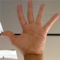
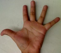
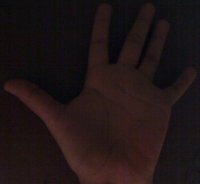
• Load the base image (src_base) and the other two test images:

  C++

      CommandLineParser parser( argc, argv, keys );
      samples::addSamplesDataSearchSubDirectory( "doc/tutorials/imgproc/histograms/histogram_comparison/images" );
      Mat src_base = imread(samples::findFile( parser.get<String>( "@input1" ) ) );
      Mat src_test1 = imread(samples::findFile( parser.get<String>( "@input2" ) ) );
      Mat src_test2 = imread(samples::findFile( parser.get<String>( "@input3" ) ) );
      if( src_base.empty() || src_test1.empty() || src_test2.empty() )
      {
          cout << "Could not open or find the images!\n" << endl;
          parser.printMessage();
          return -1;
      }

  Java

          if (args.length != 3) {
              System.err.println("You must supply 3 arguments that correspond to the paths to 3 images.");
              System.exit(0);
          }
          Mat srcBase = Imgcodecs.imread(args[0]);
          Mat srcTest1 = Imgcodecs.imread(args[1]);
          Mat srcTest2 = Imgcodecs.imread(args[2]);
          if (srcBase.empty() || srcTest1.empty() || srcTest2.empty()) {
              System.err.println("Cannot read the images");
              System.exit(0);
          }

  Python

  parser = argparse.ArgumentParser(description='Code for Histogram Comparison tutorial.')
  parser.add_argument('--input1', help='Path to input image 1.')
  parser.add_argument('--input2', help='Path to input image 2.')
  parser.add_argument('--input3', help='Path to input image 3.')
  args = parser.parse_args()
   
  src_base = cv.imread(args.input1)
  src_test1 = cv.imread(args.input2)
  src_test2 = cv.imread(args.input3)
  if src_base is None or src_test1 is None or src_test2 is None:
      print('Could not open or find the images!')
      exit(0)

• Convert them to HSV format:

  C++

      Mat hsv_base, hsv_test1, hsv_test2;
      cvtColor( src_base, hsv_base, COLOR_BGR2HSV );
      cvtColor( src_test1, hsv_test1, COLOR_BGR2HSV );
      cvtColor( src_test2, hsv_test2, COLOR_BGR2HSV );

  Java

          Mat hsvBase = new Mat(), hsvTest1 = new Mat(), hsvTest2 = new Mat();
          Imgproc.cvtColor( srcBase, hsvBase, Imgproc.COLOR_BGR2HSV );
          Imgproc.cvtColor( srcTest1, hsvTest1, Imgproc.COLOR_BGR2HSV );
          Imgproc.cvtColor( srcTest2, hsvTest2, Imgproc.COLOR_BGR2HSV );

  Python

  hsv_base = cv.cvtColor(src_base, cv.COLOR_BGR2HSV)
  hsv_test1 = cv.cvtColor(src_test1, cv.COLOR_BGR2HSV)
  hsv_test2 = cv.cvtColor(src_test2, cv.COLOR_BGR2HSV)

• Also, create an image of half the base image (in HSV format):

  C++

      Mat hsv_half_down = hsv_base( Range( hsv_base.rows/2, hsv_base.rows ), Range( 0, hsv_base.cols ) );

  Java

          Mat hsvHalfDown = hsvBase.submat( new Range( hsvBase.rows()/2, hsvBase.rows() - 1 ), new Range( 0, hsvBase.cols() - 1 ) );

  Python

  hsv_half_down = hsv_base[hsv_base.shape[0]//2:,:]

• Initialize the arguments to calculate the histograms (bins, ranges and channels H and S).

  C++

      int h_bins = 50, s_bins = 60;
      int histSize[] = { h_bins, s_bins };
   
      // hue varies from 0 to 179, saturation from 0 to 255
      float h_ranges[] = { 0, 180 };
      float s_ranges[] = { 0, 256 };
   
      const float* ranges[] = { h_ranges, s_ranges };
   
      // Use the 0-th and 1-st channels
      int channels[] = { 0, 1 };

  Java

          int hBins = 50, sBins = 60;
          int[] histSize = { hBins, sBins };
   
          // hue varies from 0 to 179, saturation from 0 to 255
          float[] ranges = { 0, 180, 0, 256 };
   
          // Use the 0-th and 1-st channels
          int[] channels = { 0, 1 };

  Python

  h_bins = 50
  s_bins = 60
  histSize = [h_bins, s_bins]
   
  # hue varies from 0 to 179, saturation from 0 to 255
  h_ranges = [0, 180]
  s_ranges = [0, 256]
  ranges = h_ranges + s_ranges # concat lists
   
  # Use the 0-th and 1-st channels
  channels = [0, 1]

• Calculate the Histograms for the base image, the 2 test images and the half-down base image:

  C++

      Mat hist_base, hist_half_down, hist_test1, hist_test2;
   
      calcHist( &hsv_base, 1, channels, Mat(), hist_base, 2, histSize, ranges, true, false );
      normalize( hist_base, hist_base, 1, 0, NORM_L1, -1, Mat() );
   
      calcHist( &hsv_half_down, 1, channels, Mat(), hist_half_down, 2, histSize, ranges, true, false );
      normalize( hist_half_down, hist_half_down, 1, 0, NORM_L1, -1, Mat() );
   
      calcHist( &hsv_test1, 1, channels, Mat(), hist_test1, 2, histSize, ranges, true, false );
      normalize( hist_test1, hist_test1, 1, 0, NORM_L1, -1, Mat() );
   
      calcHist( &hsv_test2, 1, channels, Mat(), hist_test2, 2, histSize, ranges, true, false );
      normalize( hist_test2, hist_test2, 1, 0, NORM_L1, -1, Mat() );

  Java

          Mat histBase = new Mat(), histHalfDown = new Mat(), histTest1 = new Mat(), histTest2 = new Mat();
   
          List<Mat> hsvBaseList = Arrays.asList(hsvBase);
          Imgproc.calcHist(hsvBaseList, new MatOfInt(channels), new Mat(), histBase, new MatOfInt(histSize), new MatOfFloat(ranges), false);
          Core.normalize(histBase, histBase, 1, 0, Core.NORM_L1);
   
          List<Mat> hsvHalfDownList = Arrays.asList(hsvHalfDown);
          Imgproc.calcHist(hsvHalfDownList, new MatOfInt(channels), new Mat(), histHalfDown, new MatOfInt(histSize), new MatOfFloat(ranges), false);
          Core.normalize(histHalfDown, histHalfDown, 1, 0, Core.NORM_L1);
   
          List<Mat> hsvTest1List = Arrays.asList(hsvTest1);
          Imgproc.calcHist(hsvTest1List, new MatOfInt(channels), new Mat(), histTest1, new MatOfInt(histSize), new MatOfFloat(ranges), false);
          Core.normalize(histTest1, histTest1, 1, 0, Core.NORM_L1);
   
          List<Mat> hsvTest2List = Arrays.asList(hsvTest2);
          Imgproc.calcHist(hsvTest2List, new MatOfInt(channels), new Mat(), histTest2, new MatOfInt(histSize), new MatOfFloat(ranges), false);
          Core.normalize(histTest2, histTest2, 1, 0, Core.NORM_L1);

  Python

  hist_base = cv.calcHist([hsv_base], channels, None, histSize, ranges, accumulate=False)
  cv.normalize(hist_base, hist_base, alpha=1, beta=0, norm_type=cv.NORM_L1)
   
  hist_half_down = cv.calcHist([hsv_half_down], channels, None, histSize, ranges, accumulate=False)
  cv.normalize(hist_half_down, hist_half_down, alpha=1, beta=0, norm_type=cv.NORM_L1)
   
  hist_test1 = cv.calcHist([hsv_test1], channels, None, histSize, ranges, accumulate=False)
  cv.normalize(hist_test1, hist_test1, alpha=1, beta=0, norm_type=cv.NORM_L1)
   
  hist_test2 = cv.calcHist([hsv_test2], channels, None, histSize, ranges, accumulate=False)
  cv.normalize(hist_test2, hist_test2, alpha=1, beta=0, norm_type=cv.NORM_L1)

• Apply sequentially the 6 comparison methods between the histogram of the base image (hist_base) and the other histograms:

  C++

      for( int compare_method = 0; compare_method < 6; compare_method++ )
      {
          double base_base = compareHist( hist_base, hist_base, compare_method );
          double base_half = compareHist( hist_base, hist_half_down, compare_method );
          double base_test1 = compareHist( hist_base, hist_test1, compare_method );
          double base_test2 = compareHist( hist_base, hist_test2, compare_method );
   
          cout << "Method " << compare_method << " Perfect, Base-Half, Base-Test(1), Base-Test(2) : "
               <<  base_base << " / " << base_half << " / " << base_test1 << " / " << base_test2 << endl;
      }

  Java

          for( int compareMethod = 0; compareMethod < 6; compareMethod++ ) {
              double baseBase = Imgproc.compareHist( histBase, histBase, compareMethod );
              double baseHalf = Imgproc.compareHist( histBase, histHalfDown, compareMethod );
              double baseTest1 = Imgproc.compareHist( histBase, histTest1, compareMethod );
              double baseTest2 = Imgproc.compareHist( histBase, histTest2, compareMethod );
   
              System.out.println("Method " + compareMethod + " Perfect, Base-Half, Base-Test(1), Base-Test(2) : " + baseBase + " / " + baseHalf
                      + " / " + baseTest1 + " / " + baseTest2);
          }

  Python

  for compare_method in range(6):
      base_base = cv.compareHist(hist_base, hist_base, compare_method)
      base_half = cv.compareHist(hist_base, hist_half_down, compare_method)
      base_test1 = cv.compareHist(hist_base, hist_test1, compare_method)
      base_test2 = cv.compareHist(hist_base, hist_test2, compare_method)
   
      print('Method:', compare_method, 'Perfect, Base-Half, Base-Test(1), Base-Test(2) :',\
            base_base, '/', base_half, '/', base_test1, '/', base_test2)

Results

1. We use as input the following images:

where the first one is the base (to be compared to the others), the other 2 are the test images. We will also compare the first image with respect to itself and with respect of half the base image.

1. We should expect a perfect match when we compare the base image histogram with itself. Also, compared with the histogram of half the base image, it should present a high match since both are from the same source. For the other two test images, we can observe that they have very different lighting conditions, so the matching should not be very good:

2. Here the numeric results we got with OpenCV 4.12.0:

   Method	Base - Base	Base - Half	Base - Test 1	Base - Test 2
   Correlation	1.000000	0.880438	0.20457	0.065752
   Chi-square	0.000000	0.328307	181.674	80.1494
   Intersection	1.000000	0.75005	0.315061	0.0908022
   Bhattacharyya	0.000000	0.237866	0.679825	0.873709
   Chi-Square alt.	0.000000	0.395046	2.31572	3.41024
   KL divergence	0.000000	0.321064	2.6616	9.55412

   For the Correlation and Intersection methods, the higher the metric, the more accurate the match. As we can see, the match base-base is the highest of all as expected. Also we can observe that the match base-half is the second best match (as we predicted). For the other four metrics, the less the result, the better the match.