How to use the OpenCV parallel_for_ to parallelize your code

Prev Tutorial: File Input and Output using XML and YAML files

Next Tutorial: Vectorizing your code using Universal Intrinsics

Compatibility	OpenCV >= 3.0

Goal

The goal of this tutorial is to demonstrate the use of the OpenCV parallel_for_ framework to easily parallelize your code. To illustrate the concept, we will write a program to perform convolution operation over an image. The full tutorial code is here.

Precondition

Parallel Frameworks

The first precondition is to have OpenCV built with a parallel framework. In OpenCV 4.5, the following parallel frameworks are available in that order:

• Intel Threading Building Blocks (3rdparty library, should be explicitly enabled)
• OpenMP (integrated to compiler, should be explicitly enabled)
• APPLE GCD (system wide, used automatically (APPLE only))
• Windows RT concurrency (system wide, used automatically (Windows RT only))
• Windows concurrency (part of runtime, used automatically (Windows only - MSVC++ >= 10))
• Pthreads

As you can see, several parallel frameworks can be used in the OpenCV library. Some parallel libraries are third party libraries and have to be explicitly enabled in CMake before building, while others are automatically available with the platform (e.g. APPLE GCD).

Race Conditions

Race conditions occur when more than one thread try to write or read and write to a particular memory location simultaneously. Based on that, we can broadly classify algorithms into two categories:-

1. Algorithms in which only a single thread writes data to a particular memory location.
   • In convolution, for example, even though multiple threads may read from a pixel at a particular time, only a single thread writes to a particular pixel.
2. Algorithms in which multiple threads may write to a single memory location.
   • Finding contours, features, etc. Such algorithms may require each thread to add data to a global variable simultaneously. For example, when detecting features, each thread will add features of their respective parts of the image to a common vector, thus creating a race condition.

Convolution

We will use the example of performing a convolution to demonstrate the use of parallel_for_ to parallelize the computation. This is an example of an algorithm which does not lead to a race condition.

Theory

Convolution is a simple mathematical operation widely used in image processing. Here, we slide a smaller matrix, called the kernel, over an image and a sum of the product of pixel values and corresponding values in the kernel gives us the value of the particular pixel in the output (called the anchor point of the kernel). Based on the values in the kernel, we get different results. In the example below, we use a 3x3 kernel (anchored at its center) and convolve over a 5x5 matrix to produce a 3x3 matrix. The size of the output can be altered by padding the input with suitable values.

Convolution Animation

For more information about different kernels and what they do, look here

For the purpose of this tutorial, we will implement the simplest form of the function which takes a grayscale image (1 channel) and an odd length square kernel and produces an output image. The operation will not be performed in-place.

Note

We can store a few of the relevant pixels temporarily to make sure we use the original values during the convolution and then do it in-place. However, the purpose of this tutorial is to introduce parallel_for_ function and an inplace implementation may be too complicated.

Pseudocode

InputImage src, OutputImage dst, kernel(size n)
makeborder(src, n/2)
for each pixel (i, j) strictly inside borders, do:
{
    value := 0
    for k := -n/2 to n/2, do:
        for l := -n/2 to n/2, do:
            value += kernel[n/2 + k][n/2 + l]*src[i + k][j + l]

    dst[i][j] := value
}

For an n-sized kernel, we will add a border of size n/2 to handle edge cases. We then run two loops to move along the kernel and add the products to sum

Implementation

Sequential implementation

void conv_seq(Mat src, Mat &dst, Mat kernel)
{
 int rows = src.rows, cols = src.cols;
 dst = Mat(rows, cols, src.type());

 // Taking care of edge values
 // Make border = kernel.rows / 2;

 int sz = kernel.rows / 2;
 copyMakeBorder(src, src, sz, sz, sz, sz, BORDER_REPLICATE);

 for (int i = 0; i < rows; i++)
 {
 uchar *dptr = dst.ptr(i);
 for (int j = 0; j < cols; j++)
 {
 double value = 0;

 for (int k = -sz; k <= sz; k++)
 {
 // slightly faster results when we create a ptr due to more efficient memory access.
 uchar *sptr = src.ptr(i + sz + k);
 for (int l = -sz; l <= sz; l++)
 {
 value += kernel.ptr<double>(k + sz)[l + sz] * sptr[j + sz + l];
 }
 }
 dptr[j] = saturate_cast<uchar>(value);
 }
 }
}

We first make an output matrix(dst) with the same size as src and add borders to the src image(to handle edge cases).

 int rows = src.rows, cols = src.cols;
 dst = Mat(rows, cols, src.type());

 // Taking care of edge values
 // Make border = kernel.rows / 2;

 int sz = kernel.rows / 2;
 copyMakeBorder(src, src, sz, sz, sz, sz, BORDER_REPLICATE);

We then sequentially iterate over the pixels in the src image and compute the value over the kernel and the neighbouring pixel values. We then fill value to the corresponding pixel in the dst image.

 for (int i = 0; i < rows; i++)
 {
 uchar *dptr = dst.ptr(i);
 for (int j = 0; j < cols; j++)
 {
 double value = 0;

 for (int k = -sz; k <= sz; k++)
 {
 // slightly faster results when we create a ptr due to more efficient memory access.
 uchar *sptr = src.ptr(i + sz + k);
 for (int l = -sz; l <= sz; l++)
 {
 value += kernel.ptr<double>(k + sz)[l + sz] * sptr[j + sz + l];
 }
 }
 dptr[j] = saturate_cast<uchar>(value);
 }
 }

Parallel implementation

When looking at the sequential implementation, we can notice that each pixel depends on multiple neighbouring pixels but only one pixel is edited at a time. Thus, to optimize the computation, we can split the image into stripes and parallely perform convolution on each, by exploiting the multi-core architecture of modern processor. The OpenCV cv::parallel_for_ framework automatically decides how to split the computation efficiently and does most of the work for us.

Note

Although values of a pixel in a particular stripe may depend on pixel values outside the stripe, these are only read only operations and hence will not cause undefined behaviour.

We first declare a custom class that inherits from cv::ParallelLoopBody and override the virtual void operator ()(const cv::Range& range) const.

class parallelConvolution : public ParallelLoopBody
{
private:
 Mat m_src, &m_dst;
 Mat m_kernel;
 int sz;

public:
 parallelConvolution(Mat src, Mat &dst, Mat kernel)
 : m_src(src), m_dst(dst), m_kernel(kernel)
 {
 sz = kernel.rows / 2;
 }

 virtual void operator()(const Range &range) const CV_OVERRIDE
 {
 for (int r = range.start; r < range.end; r++)
 {
 int i = r / m_src.cols, j = r % m_src.cols;

 double value = 0;
 for (int k = -sz; k <= sz; k++)
 {
 uchar *sptr = m_src.ptr(i + sz + k);
 for (int l = -sz; l <= sz; l++)
 {
 value += m_kernel.ptr<double>(k + sz)[l + sz] * sptr[j + sz + l];
 }
 }
 m_dst.ptr(i)[j] = saturate_cast<uchar>(value);
 }
 }
};

The range in the operator () represents the subset of values that will be treated by an individual thread. Based on the requirement, there may be different ways of splitting the range which in turn changes the computation.

For example, we can either

1. Split the entire traversal of the image and obtain the [row, col] coordinate in the following way (as shown in the above code):

    virtual void operator()(const Range &range) const CV_OVERRIDE
    {
    for (int r = range.start; r < range.end; r++)
    {
    int i = r / m_src.cols, j = r % m_src.cols;
   
    double value = 0;
    for (int k = -sz; k <= sz; k++)
    {
    uchar *sptr = m_src.ptr(i + sz + k);
    for (int l = -sz; l <= sz; l++)
    {
    value += m_kernel.ptr<double>(k + sz)[l + sz] * sptr[j + sz + l];
    }
    }
    m_dst.ptr(i)[j] = saturate_cast<uchar>(value);
    }
    }

   We would then call the parallel_for_ function in the following way:

    parallelConvolution obj(src, dst, kernel);
    parallel_for_(Range(0, rows * cols), obj);

   
   

2. Split the rows and compute for each row:

    virtual void operator()(const Range &range) const CV_OVERRIDE
    {
    for (int i = range.start; i < range.end; i++)
    {
   
    uchar *dptr = dst.ptr(i);
    for (int j = 0; j < cols; j++)
    {
    double value = 0;
    for (int k = -sz; k <= sz; k++)
    {
    uchar *sptr = src.ptr(i + sz + k);
    for (int l = -sz; l <= sz; l++)
    {
    value += kernel.ptr<double>(k + sz)[l + sz] * sptr[j + sz + l];
    }
    }
    dptr[j] = saturate_cast<uchar>(value);
    }
    }
    }

   In this case, we call the parallel_for_ function with a different range:

    parallelConvolutionRowSplit obj(src, dst, kernel);
    parallel_for_(Range(0, rows), obj);

   Note

   In our case, both implementations perform similarly. Some cases may allow better memory access patterns or other performance benefits.

   To set the number of threads, you can use: cv::setNumThreads. You can also specify the number of splitting using the nstripes parameter in cv::parallel_for_. For instance, if your processor has 4 threads, setting cv::setNumThreads(2) or setting nstripes=2 should be the same as by default it will use all the processor threads available but will split the workload only on two threads.

Note

C++ 11 standard allows to simplify the parallel implementation by get rid of the parallelConvolution class and replacing it with lambda expression:

 parallel_for_(Range(0, rows * cols), [&](const Range &range)
 {
 for (int r = range.start; r < range.end; r++)
 {
 int i = r / cols, j = r % cols;

 double value = 0;
 for (int k = -sz; k <= sz; k++)
 {
 uchar *sptr = src.ptr(i + sz + k);
 for (int l = -sz; l <= sz; l++)
 {
 value += kernel.ptr<double>(k + sz)[l + sz] * sptr[j + sz + l];
 }
 }
 dst.ptr(i)[j] = saturate_cast<uchar>(value);
 }
 });

Results

The resulting time taken for execution of the two implementations on a

• 512x512 input with a 5x5 kernel:

    This program shows how to use the OpenCV parallel_for_ function and
    compares the performance of the sequential and parallel implementations for a
    convolution operation
    Usage:
    ./a.out [image_path -- default lena.jpg]
  
    Sequential Implementation: 0.0953564s
    Parallel Implementation: 0.0246762s
    Parallel Implementation(Row Split): 0.0248722s
  

• 512x512 input with a 3x3 kernel

    This program shows how to use the OpenCV parallel_for_ function and
    compares the performance of the sequential and parallel implementations for a
    convolution operation
    Usage:
    ./a.out [image_path -- default lena.jpg]
  
    Sequential Implementation: 0.0301325s
    Parallel Implementation: 0.0117053s
    Parallel Implementation(Row Split): 0.0117894s
  

The performance of the parallel implementation depends on the type of CPU you have. For instance, on 4 cores - 8 threads CPU, runtime may be 6x to 7x faster than a sequential implementation. There are many factors to explain why we do not achieve a speed-up of 8x:

• the overhead to create and manage the threads,
• background processes running in parallel,
• the difference between 4 hardware cores with 2 logical threads for each core and 8 hardware cores.

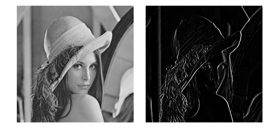
In the tutorial, we used a horizontal gradient filter(as shown in the animation above), which produces an image highlighting the vertical edges.

result image