Anisotropic image segmentation by a gradient structure tensor

Prev Tutorial: Motion Deblur Filter

Next Tutorial: Periodic Noise Removing Filter

Original author	Karpushin Vladislav
Compatibility	OpenCV >= 3.0

Goal

In this tutorial you will learn:

• what the gradient structure tensor is
• how to estimate orientation and coherency of an anisotropic image by a gradient structure tensor
• how to segment an anisotropic image with a single local orientation by a gradient structure tensor

Theory

Note

The explanation is based on the books [120], [22] and [260]. Good physical explanation of a gradient structure tensor is given in [284]. Also, you can refer to a wikipedia page Structure tensor.

A anisotropic image on this page is a real world image.

What is the gradient structure tensor?

In mathematics, the gradient structure tensor (also referred to as the second-moment matrix, the second order moment tensor, the inertia tensor, etc.) is a matrix derived from the gradient of a function. It summarizes the predominant directions of the gradient in a specified neighborhood of a point, and the degree to which those directions are coherent (coherency). The gradient structure tensor is widely used in image processing and computer vision for 2D/3D image segmentation, motion detection, adaptive filtration, local image features detection, etc.

Important features of anisotropic images include orientation and coherency of a local anisotropy. In this paper we will show how to estimate orientation and coherency, and how to segment an anisotropic image with a single local orientation by a gradient structure tensor.

The gradient structure tensor of an image is a 2x2 symmetric matrix. Eigenvectors of the gradient structure tensor indicate local orientation, whereas eigenvalues give coherency (a measure of anisotropism).

The gradient structure tensor \(J\) of an image \(Z\) can be written as:

\[J = \begin{bmatrix} J_{11} & J_{12} \\ J_{12} & J_{22} \end{bmatrix}\]

where \(J_{11} = M[Z_{x}^{2}]\), \(J_{22} = M[Z_{y}^{2}]\), \(J_{12} = M[Z_{x}Z_{y}]\) - components of the tensor, \(M[]\) is a symbol of mathematical expectation (we can consider this operation as averaging in a window w), \(Z_{x}\) and \(Z_{y}\) are partial derivatives of an image \(Z\) with respect to \(x\) and \(y\).

The eigenvalues of the tensor can be found in the below formula:

\[\lambda_{1,2} = \frac{1}{2} \left [ J_{11} + J_{22} \pm \sqrt{(J_{11} - J_{22})^{2} + 4J_{12}^{2}} \right ] \]

where \(\lambda_1\) - largest eigenvalue, \(\lambda_2\) - smallest eigenvalue.

How to estimate orientation and coherency of an anisotropic image by gradient structure tensor?

The orientation of an anisotropic image:

\[\alpha = 0.5arctg\frac{2J_{12}}{J_{22} - J_{11}}\]

Coherency:

\[C = \frac{\lambda_1 - \lambda_2}{\lambda_1 + \lambda_2}\]

The coherency ranges from 0 to 1. For ideal local orientation ( \(\lambda_2\) = 0, \(\lambda_1\) > 0) it is one, for an isotropic gray value structure ( \(\lambda_1\) = \(\lambda_2\) > 0) it is zero.

Source code

You can find source code in the samples/cpp/tutorial_code/ImgProc/anisotropic_image_segmentation/anisotropic_image_segmentation.cpp of the OpenCV source code library.

C++

#include <iostream>
#include "opencv2/imgproc.hpp"
#include "opencv2/imgcodecs.hpp"

using namespace cv;
using namespace std;

void calcGST(const Mat& inputImg, Mat& imgCoherencyOut, Mat& imgOrientationOut, int w);

int main()
{
    int W = 52;             // window size is WxW
    double C_Thr = 0.43;    // threshold for coherency
    int LowThr = 35;        // threshold1 for orientation, it ranges from 0 to 180
    int HighThr = 57;       // threshold2 for orientation, it ranges from 0 to 180

    Mat imgIn = imread("input.jpg", IMREAD_GRAYSCALE);
    if (imgIn.empty()) //check whether the image is loaded or not
    {
        cout << "ERROR : Image cannot be loaded..!!" << endl;
        return -1;
    }

    Mat imgCoherency, imgOrientation;
    calcGST(imgIn, imgCoherency, imgOrientation, W);

    Mat imgCoherencyBin;
    imgCoherencyBin = imgCoherency > C_Thr;
    Mat imgOrientationBin;
    inRange(imgOrientation, Scalar(LowThr), Scalar(HighThr), imgOrientationBin);

    Mat imgBin;
    imgBin = imgCoherencyBin & imgOrientationBin;

    normalize(imgCoherency, imgCoherency, 0, 255, NORM_MINMAX);
    normalize(imgOrientation, imgOrientation, 0, 255, NORM_MINMAX);

    imwrite("result.jpg", 0.5*(imgIn + imgBin));
    imwrite("Coherency.jpg", imgCoherency);
    imwrite("Orientation.jpg", imgOrientation);
    return 0;
}
void calcGST(const Mat& inputImg, Mat& imgCoherencyOut, Mat& imgOrientationOut, int w)
{
    Mat img;
    inputImg.convertTo(img, CV_32F);

    // GST components calculation (start)
    // J =  (J11 J12; J12 J22) - GST
    Mat imgDiffX, imgDiffY, imgDiffXY;
    Sobel(img, imgDiffX, CV_32F, 1, 0, 3);
    Sobel(img, imgDiffY, CV_32F, 0, 1, 3);
    multiply(imgDiffX, imgDiffY, imgDiffXY);

    Mat imgDiffXX, imgDiffYY;
    multiply(imgDiffX, imgDiffX, imgDiffXX);
    multiply(imgDiffY, imgDiffY, imgDiffYY);

    Mat J11, J22, J12;      // J11, J22 and J12 are GST components
    boxFilter(imgDiffXX, J11, CV_32F, Size(w, w));
    boxFilter(imgDiffYY, J22, CV_32F, Size(w, w));
    boxFilter(imgDiffXY, J12, CV_32F, Size(w, w));
    // GST components calculation (stop)

    // eigenvalue calculation (start)
    // lambda1 = 0.5*(J11 + J22 + sqrt((J11-J22)^2 + 4*J12^2))
    // lambda2 = 0.5*(J11 + J22 - sqrt((J11-J22)^2 + 4*J12^2))
    Mat tmp1, tmp2, tmp3, tmp4;
    tmp1 = J11 + J22;
    tmp2 = J11 - J22;
    multiply(tmp2, tmp2, tmp2);
    multiply(J12, J12, tmp3);
    sqrt(tmp2 + 4.0 * tmp3, tmp4);

    Mat lambda1, lambda2;
    lambda1 = tmp1 + tmp4;
    lambda1 = 0.5*lambda1;      // biggest eigenvalue
    lambda2 = tmp1 - tmp4;
    lambda2 = 0.5*lambda2;      // smallest eigenvalue
    // eigenvalue calculation (stop)

    // Coherency calculation (start)
    // Coherency = (lambda1 - lambda2)/(lambda1 + lambda2)) - measure of anisotropism
    // Coherency is anisotropy degree (consistency of local orientation)
    divide(lambda1 - lambda2, lambda1 + lambda2, imgCoherencyOut);
    // Coherency calculation (stop)

    // orientation angle calculation (start)
    // tan(2*Alpha) = 2*J12/(J22 - J11)
    // Alpha = 0.5 atan2(2*J12/(J22 - J11))
    phase(J22 - J11, 2.0*J12, imgOrientationOut, true);
    imgOrientationOut = 0.5*imgOrientationOut;
    // orientation angle calculation (stop)
}

Python

import cv2 as cv
import numpy as np
import argparse

W = 52          # window size is WxW
C_Thr = 0.43    # threshold for coherency
LowThr = 35     # threshold1 for orientation, it ranges from 0 to 180
HighThr = 57    # threshold2 for orientation, it ranges from 0 to 180


def calcGST(inputIMG, w):

    img = inputIMG.astype(np.float32)

    # GST components calculation (start)
    # J =  (J11 J12; J12 J22) - GST
    imgDiffX = cv.Sobel(img, cv.CV_32F, 1, 0, 3)
    imgDiffY = cv.Sobel(img, cv.CV_32F, 0, 1, 3)
    imgDiffXY = cv.multiply(imgDiffX, imgDiffY)
    

    imgDiffXX = cv.multiply(imgDiffX, imgDiffX)
    imgDiffYY = cv.multiply(imgDiffY, imgDiffY)

    J11 = cv.boxFilter(imgDiffXX, cv.CV_32F, (w,w))
    J22 = cv.boxFilter(imgDiffYY, cv.CV_32F, (w,w))
    J12 = cv.boxFilter(imgDiffXY, cv.CV_32F, (w,w))
    # GST components calculations (stop)

    # eigenvalue calculation (start)
    # lambda1 = 0.5*(J11 + J22 + sqrt((J11-J22)^2 + 4*J12^2))
    # lambda2 = 0.5*(J11 + J22 - sqrt((J11-J22)^2 + 4*J12^2))
    tmp1 = J11 + J22
    tmp2 = J11 - J22
    tmp2 = cv.multiply(tmp2, tmp2)
    tmp3 = cv.multiply(J12, J12)
    tmp4 = np.sqrt(tmp2 + 4.0 * tmp3)

    lambda1 = 0.5*(tmp1 + tmp4)    # biggest eigenvalue
    lambda2 = 0.5*(tmp1 - tmp4)    # smallest eigenvalue
    # eigenvalue calculation (stop)

    # Coherency calculation (start)
    # Coherency = (lambda1 - lambda2)/(lambda1 + lambda2)) - measure of anisotropism
    # Coherency is anisotropy degree (consistency of local orientation)
    imgCoherencyOut = cv.divide(lambda1 - lambda2, lambda1 + lambda2)
    # Coherency calculation (stop)

    # orientation angle calculation (start)
    # tan(2*Alpha) = 2*J12/(J22 - J11)
    # Alpha = 0.5 atan2(2*J12/(J22 - J11))
    imgOrientationOut = cv.phase(J22 - J11, 2.0 * J12, angleInDegrees = True)
    imgOrientationOut = 0.5 * imgOrientationOut
    # orientation angle calculation (stop)

    return imgCoherencyOut, imgOrientationOut


parser = argparse.ArgumentParser(description='Code for Anisotropic image segmentation tutorial.')
parser.add_argument('-i', '--input', help='Path to input image.', required=True)
args = parser.parse_args()

imgIn = cv.imread(args.input, cv.IMREAD_GRAYSCALE)
if imgIn is None:
    print('Could not open or find the image: {}'.format(args.input))
    exit(0)


imgCoherency, imgOrientation = calcGST(imgIn, W)


_, imgCoherencyBin = cv.threshold(imgCoherency, C_Thr, 255, cv.THRESH_BINARY)
_, imgOrientationBin = cv.threshold(imgOrientation, LowThr, HighThr, cv.THRESH_BINARY)



imgBin = cv.bitwise_and(imgCoherencyBin, imgOrientationBin)


imgCoherency = cv.normalize(imgCoherency, None, alpha=0, beta=1, norm_type=cv.NORM_MINMAX, dtype=cv.CV_32F)
imgOrientation = cv.normalize(imgOrientation, None, alpha=0, beta=1, norm_type=cv.NORM_MINMAX, dtype=cv.CV_32F)

cv.imshow('result.jpg', np.uint8(0.5*(imgIn + imgBin)))
cv.imshow('Coherency.jpg', imgCoherency)
cv.imshow('Orientation.jpg', imgOrientation)
cv.waitKey(0)

Explanation

An anisotropic image segmentation algorithm consists of a gradient structure tensor calculation, an orientation calculation, a coherency calculation and an orientation and coherency thresholding:

C++

    Mat imgCoherency, imgOrientation;
    calcGST(imgIn, imgCoherency, imgOrientation, W);

    Mat imgCoherencyBin;
    imgCoherencyBin = imgCoherency > C_Thr;
    Mat imgOrientationBin;
    inRange(imgOrientation, Scalar(LowThr), Scalar(HighThr), imgOrientationBin);

    Mat imgBin;
    imgBin = imgCoherencyBin & imgOrientationBin;

Python

imgCoherency, imgOrientation = calcGST(imgIn, W)


_, imgCoherencyBin = cv.threshold(imgCoherency, C_Thr, 255, cv.THRESH_BINARY)
_, imgOrientationBin = cv.threshold(imgOrientation, LowThr, HighThr, cv.THRESH_BINARY)



imgBin = cv.bitwise_and(imgCoherencyBin, imgOrientationBin)

A function calcGST() calculates orientation and coherency by using a gradient structure tensor. An input parameter w defines a window size:

C++

void calcGST(const Mat& inputImg, Mat& imgCoherencyOut, Mat& imgOrientationOut, int w)
{
    Mat img;
    inputImg.convertTo(img, CV_32F);

    // GST components calculation (start)
    // J =  (J11 J12; J12 J22) - GST
    Mat imgDiffX, imgDiffY, imgDiffXY;
    Sobel(img, imgDiffX, CV_32F, 1, 0, 3);
    Sobel(img, imgDiffY, CV_32F, 0, 1, 3);
    multiply(imgDiffX, imgDiffY, imgDiffXY);

    Mat imgDiffXX, imgDiffYY;
    multiply(imgDiffX, imgDiffX, imgDiffXX);
    multiply(imgDiffY, imgDiffY, imgDiffYY);

    Mat J11, J22, J12;      // J11, J22 and J12 are GST components
    boxFilter(imgDiffXX, J11, CV_32F, Size(w, w));
    boxFilter(imgDiffYY, J22, CV_32F, Size(w, w));
    boxFilter(imgDiffXY, J12, CV_32F, Size(w, w));
    // GST components calculation (stop)

    // eigenvalue calculation (start)
    // lambda1 = 0.5*(J11 + J22 + sqrt((J11-J22)^2 + 4*J12^2))
    // lambda2 = 0.5*(J11 + J22 - sqrt((J11-J22)^2 + 4*J12^2))
    Mat tmp1, tmp2, tmp3, tmp4;
    tmp1 = J11 + J22;
    tmp2 = J11 - J22;
    multiply(tmp2, tmp2, tmp2);
    multiply(J12, J12, tmp3);
    sqrt(tmp2 + 4.0 * tmp3, tmp4);

    Mat lambda1, lambda2;
    lambda1 = tmp1 + tmp4;
    lambda1 = 0.5*lambda1;      // biggest eigenvalue
    lambda2 = tmp1 - tmp4;
    lambda2 = 0.5*lambda2;      // smallest eigenvalue
    // eigenvalue calculation (stop)

    // Coherency calculation (start)
    // Coherency = (lambda1 - lambda2)/(lambda1 + lambda2)) - measure of anisotropism
    // Coherency is anisotropy degree (consistency of local orientation)
    divide(lambda1 - lambda2, lambda1 + lambda2, imgCoherencyOut);
    // Coherency calculation (stop)

    // orientation angle calculation (start)
    // tan(2*Alpha) = 2*J12/(J22 - J11)
    // Alpha = 0.5 atan2(2*J12/(J22 - J11))
    phase(J22 - J11, 2.0*J12, imgOrientationOut, true);
    imgOrientationOut = 0.5*imgOrientationOut;
    // orientation angle calculation (stop)
}

Python

def calcGST(inputIMG, w):

    img = inputIMG.astype(np.float32)

    # GST components calculation (start)
    # J =  (J11 J12; J12 J22) - GST
    imgDiffX = cv.Sobel(img, cv.CV_32F, 1, 0, 3)
    imgDiffY = cv.Sobel(img, cv.CV_32F, 0, 1, 3)
    imgDiffXY = cv.multiply(imgDiffX, imgDiffY)
    

    imgDiffXX = cv.multiply(imgDiffX, imgDiffX)
    imgDiffYY = cv.multiply(imgDiffY, imgDiffY)

    J11 = cv.boxFilter(imgDiffXX, cv.CV_32F, (w,w))
    J22 = cv.boxFilter(imgDiffYY, cv.CV_32F, (w,w))
    J12 = cv.boxFilter(imgDiffXY, cv.CV_32F, (w,w))
    # GST components calculations (stop)

    # eigenvalue calculation (start)
    # lambda1 = 0.5*(J11 + J22 + sqrt((J11-J22)^2 + 4*J12^2))
    # lambda2 = 0.5*(J11 + J22 - sqrt((J11-J22)^2 + 4*J12^2))
    tmp1 = J11 + J22
    tmp2 = J11 - J22
    tmp2 = cv.multiply(tmp2, tmp2)
    tmp3 = cv.multiply(J12, J12)
    tmp4 = np.sqrt(tmp2 + 4.0 * tmp3)

    lambda1 = 0.5*(tmp1 + tmp4)    # biggest eigenvalue
    lambda2 = 0.5*(tmp1 - tmp4)    # smallest eigenvalue
    # eigenvalue calculation (stop)

    # Coherency calculation (start)
    # Coherency = (lambda1 - lambda2)/(lambda1 + lambda2)) - measure of anisotropism
    # Coherency is anisotropy degree (consistency of local orientation)
    imgCoherencyOut = cv.divide(lambda1 - lambda2, lambda1 + lambda2)
    # Coherency calculation (stop)

    # orientation angle calculation (start)
    # tan(2*Alpha) = 2*J12/(J22 - J11)
    # Alpha = 0.5 atan2(2*J12/(J22 - J11))
    imgOrientationOut = cv.phase(J22 - J11, 2.0 * J12, angleInDegrees = True)
    imgOrientationOut = 0.5 * imgOrientationOut
    # orientation angle calculation (stop)

    return imgCoherencyOut, imgOrientationOut

The below code applies a thresholds LowThr and HighThr to image orientation and a threshold C_Thr to image coherency calculated by the previous function. LowThr and HighThr define orientation range:

C++

    Mat imgCoherencyBin;
    imgCoherencyBin = imgCoherency > C_Thr;
    Mat imgOrientationBin;
    inRange(imgOrientation, Scalar(LowThr), Scalar(HighThr), imgOrientationBin);

Python

_, imgCoherencyBin = cv.threshold(imgCoherency, C_Thr, 255, cv.THRESH_BINARY)
_, imgOrientationBin = cv.threshold(imgOrientation, LowThr, HighThr, cv.THRESH_BINARY)

And finally we combine thresholding results:

C++

    Mat imgBin;
    imgBin = imgCoherencyBin & imgOrientationBin;

Python

imgBin = cv.bitwise_and(imgCoherencyBin, imgOrientationBin)

Result

Below you can see the real anisotropic image with single direction:

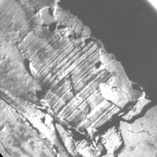
Anisotropic image with the single direction

Below you can see the orientation and coherency of the anisotropic image:

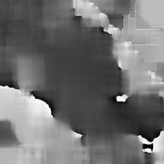
Orientation

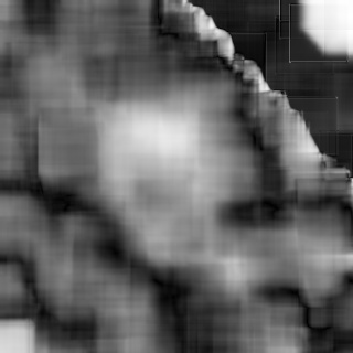
Coherency

Below you can see the segmentation result:

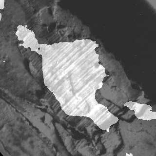
Segmentation result

The result has been computed with w = 52, C_Thr = 0.43, LowThr = 35, HighThr = 57. We can see that the algorithm selected only the areas with one single direction.

References

• Structure tensor - structure tensor description on the wikipedia