|
OpenCV
4.5.1
Open Source Computer Vision
|
|
OpenCV
4.5.1
Open Source Computer Vision
|
OpenCV provides two transformation functions, cv.warpAffine and cv.warpPerspective, with which you can perform all kinds of transformations. cv.warpAffine takes a 2x3 transformation matrix while cv.warpPerspective takes a 3x3 transformation matrix as input.
Scaling is just resizing of the image. OpenCV comes with a function cv.resize() for this purpose. The size of the image can be specified manually, or you can specify the scaling factor. Different interpolation methods are used. Preferable interpolation methods are cv.INTER_AREA for shrinking and cv.INTER_CUBIC (slow) & cv.INTER_LINEAR for zooming. By default, the interpolation method cv.INTER_LINEAR is used for all resizing purposes. You can resize an input image with either of following methods:
Translation is the shifting of an object's location. If you know the shift in the (x,y) direction and let it be \((t_x,t_y)\), you can create the transformation matrix \(\textbf{M}\) as follows:
\[M = \begin{bmatrix} 1 & 0 & t_x \\ 0 & 1 & t_y \end{bmatrix}\]
You can take make it into a Numpy array of type np.float32 and pass it into the cv.warpAffine() function. See the below example for a shift of (100,50):
warning
The third argument of the cv.warpAffine() function is the size of the output image, which should be in the form of **(width, height)**. Remember width = number of columns, and height = number of rows.
See the result below:

Rotation of an image for an angle \(\theta\) is achieved by the transformation matrix of the form
\[M = \begin{bmatrix} cos\theta & -sin\theta \\ sin\theta & cos\theta \end{bmatrix}\]
But OpenCV provides scaled rotation with adjustable center of rotation so that you can rotate at any location you prefer. The modified transformation matrix is given by
\[\begin{bmatrix} \alpha & \beta & (1- \alpha ) \cdot center.x - \beta \cdot center.y \\ - \beta & \alpha & \beta \cdot center.x + (1- \alpha ) \cdot center.y \end{bmatrix}\]
where:
\[\begin{array}{l} \alpha = scale \cdot \cos \theta , \\ \beta = scale \cdot \sin \theta \end{array}\]
To find this transformation matrix, OpenCV provides a function, cv.getRotationMatrix2D. Check out the below example which rotates the image by 90 degree with respect to center without any scaling.
See the result:

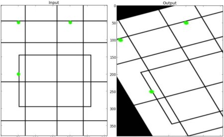
In affine transformation, all parallel lines in the original image will still be parallel in the output image. To find the transformation matrix, we need three points from the input image and their corresponding locations in the output image. Then cv.getAffineTransform will create a 2x3 matrix which is to be passed to cv.warpAffine.
Check the below example, and also look at the points I selected (which are marked in green color):
See the result:
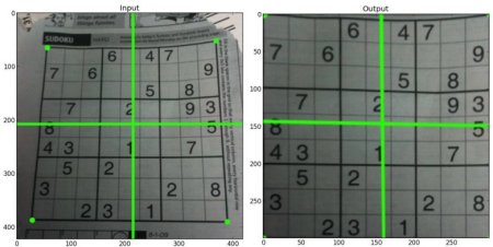
For perspective transformation, you need a 3x3 transformation matrix. Straight lines will remain straight even after the transformation. To find this transformation matrix, you need 4 points on the input image and corresponding points on the output image. Among these 4 points, 3 of them should not be collinear. Then the transformation matrix can be found by the function cv.getPerspectiveTransform. Then apply cv.warpPerspective with this 3x3 transformation matrix.
See the code below:
Result:
 1.8.13