 |
OpenCV
3.4.2
Open Source Computer Vision
|
 |
OpenCV
3.4.2
Open Source Computer Vision
|
Cameras have been around for a long-long time. However, with the introduction of the cheap pinhole cameras in the late 20th century, they became a common occurrence in our everyday life. Unfortunately, this cheapness comes with its price: significant distortion. Luckily, these are constants and with a calibration and some remapping we can correct this. Furthermore, with calibration you may also determine the relation between the camera's natural units (pixels) and the real world units (for example millimeters).
For the distortion OpenCV takes into account the radial and tangential factors. For the radial factor one uses the following formula:
\[x_{distorted} = x( 1 + k_1 r^2 + k_2 r^4 + k_3 r^6) \\ y_{distorted} = y( 1 + k_1 r^2 + k_2 r^4 + k_3 r^6)\]
So for an undistorted pixel point at \((x,y)\) coordinates, its position on the distorted image will be \((x_{distorted} y_{distorted})\). The presence of the radial distortion manifests in form of the "barrel" or "fish-eye" effect.
Tangential distortion occurs because the image taking lenses are not perfectly parallel to the imaging plane. It can be represented via the formulas:
\[x_{distorted} = x + [ 2p_1xy + p_2(r^2+2x^2)] \\ y_{distorted} = y + [ p_1(r^2+ 2y^2)+ 2p_2xy]\]
So we have five distortion parameters which in OpenCV are presented as one row matrix with 5 columns:
\[distortion\_coefficients=(k_1 \hspace{10pt} k_2 \hspace{10pt} p_1 \hspace{10pt} p_2 \hspace{10pt} k_3)\]
Now for the unit conversion we use the following formula:
\[\left [ \begin{matrix} x \\ y \\ w \end{matrix} \right ] = \left [ \begin{matrix} f_x & 0 & c_x \\ 0 & f_y & c_y \\ 0 & 0 & 1 \end{matrix} \right ] \left [ \begin{matrix} X \\ Y \\ Z \end{matrix} \right ]\]
Here the presence of \(w\) is explained by the use of homography coordinate system (and \(w=Z\)). The unknown parameters are \(f_x\) and \(f_y\) (camera focal lengths) and \((c_x, c_y)\) which are the optical centers expressed in pixels coordinates. If for both axes a common focal length is used with a given \(a\) aspect ratio (usually 1), then \(f_y=f_x*a\) and in the upper formula we will have a single focal length \(f\). The matrix containing these four parameters is referred to as the camera matrix. While the distortion coefficients are the same regardless of the camera resolutions used, these should be scaled along with the current resolution from the calibrated resolution.
The process of determining these two matrices is the calibration. Calculation of these parameters is done through basic geometrical equations. The equations used depend on the chosen calibrating objects. Currently OpenCV supports three types of objects for calibration:
Basically, you need to take snapshots of these patterns with your camera and let OpenCV find them. Each found pattern results in a new equation. To solve the equation you need at least a predetermined number of pattern snapshots to form a well-posed equation system. This number is higher for the chessboard pattern and less for the circle ones. For example, in theory the chessboard pattern requires at least two snapshots. However, in practice we have a good amount of noise present in our input images, so for good results you will probably need at least 10 good snapshots of the input pattern in different positions.
The sample application will:
You may also find the source code in the samples/cpp/tutorial_code/calib3d/camera_calibration/ folder of the OpenCV source library or download it from here. The program has a single argument: the name of its configuration file. If none is given then it will try to open the one named "default.xml". Here's a sample configuration file in XML format. In the configuration file you may choose to use camera as an input, a video file or an image list. If you opt for the last one, you will need to create a configuration file where you enumerate the images to use. Here's an example of this. The important part to remember is that the images need to be specified using the absolute path or the relative one from your application's working directory. You may find all this in the samples directory mentioned above.
The application starts up with reading the settings from the configuration file. Although, this is an important part of it, it has nothing to do with the subject of this tutorial: camera calibration. Therefore, I've chosen not to post the code for that part here. Technical background on how to do this you can find in the File Input and Output using XML and YAML files tutorial.
Get next input, if it fails or we have enough of them - calibrate
After this we have a big loop where we do the following operations: get the next image from the image list, camera or video file. If this fails or we have enough images then we run the calibration process. In case of image we step out of the loop and otherwise the remaining frames will be undistorted (if the option is set) via changing from DETECTION mode to the CALIBRATED one.
For some cameras we may need to flip the input image. Here we do this too.
Find the pattern in the current input
The formation of the equations I mentioned above aims to finding major patterns in the input: in case of the chessboard this are corners of the squares and for the circles, well, the circles themselves. The position of these will form the result which will be written into the pointBuf vector.
Depending on the type of the input pattern you use either the cv::findChessboardCorners or the cv::findCirclesGrid function. For both of them you pass the current image and the size of the board and you'll get the positions of the patterns. Furthermore, they return a boolean variable which states if the pattern was found in the input (we only need to take into account those images where this is true!).
Then again in case of cameras we only take camera images when an input delay time is passed. This is done in order to allow user moving the chessboard around and getting different images. Similar images result in similar equations, and similar equations at the calibration step will form an ill-posed problem, so the calibration will fail. For square images the positions of the corners are only approximate. We may improve this by calling the cv::cornerSubPix function. It will produce better calibration result. After this we add a valid inputs result to the imagePoints vector to collect all of the equations into a single container. Finally, for visualization feedback purposes we will draw the found points on the input image using cv::findChessboardCorners function.
Show state and result to the user, plus command line control of the application
This part shows text output on the image.
If we ran calibration and got camera's matrix with the distortion coefficients we may want to correct the image using cv::undistort function:
Then we show the image and wait for an input key and if this is u we toggle the distortion removal, if it is g we start again the detection process, and finally for the ESC key we quit the application:
Show the distortion removal for the images too
When you work with an image list it is not possible to remove the distortion inside the loop. Therefore, you must do this after the loop. Taking advantage of this now I'll expand the cv::undistort function, which is in fact first calls cv::initUndistortRectifyMap to find transformation matrices and then performs transformation using cv::remap function. Because, after successful calibration map calculation needs to be done only once, by using this expanded form you may speed up your application:
Because the calibration needs to be done only once per camera, it makes sense to save it after a successful calibration. This way later on you can just load these values into your program. Due to this we first make the calibration, and if it succeeds we save the result into an OpenCV style XML or YAML file, depending on the extension you give in the configuration file.
Therefore in the first function we just split up these two processes. Because we want to save many of the calibration variables we'll create these variables here and pass on both of them to the calibration and saving function. Again, I'll not show the saving part as that has little in common with the calibration. Explore the source file in order to find out how and what:
We do the calibration with the help of the cv::calibrateCamera function. It has the following parameters:
Let there be this input chessboard pattern which has a size of 9 X 6. I've used an AXIS IP camera to create a couple of snapshots of the board and saved it into VID5 directory. I've put this inside the images/CameraCalibration folder of my working directory and created the following VID5.XML file that describes which images to use:
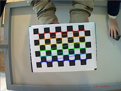
Then passed images/CameraCalibration/VID5/VID5.XML as an input in the configuration file. Here's a chessboard pattern found during the runtime of the application:

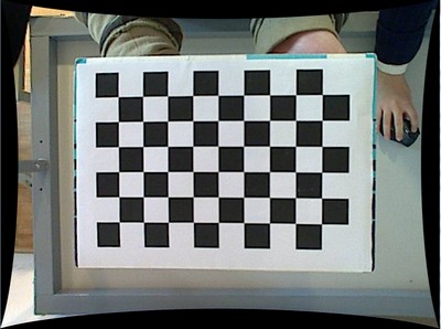
After applying the distortion removal we get:

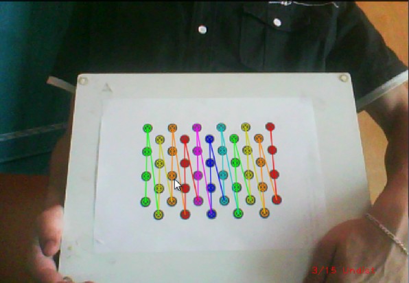
The same works for this asymmetrical circle pattern by setting the input width to 4 and height to 11. This time I've used a live camera feed by specifying its ID ("1") for the input. Here's, how a detected pattern should look:

In both cases in the specified output XML/YAML file you'll find the camera and distortion coefficients matrices:
Add these values as constants to your program, call the cv::initUndistortRectifyMap and the cv::remap function to remove distortion and enjoy distortion free inputs for cheap and low quality cameras.
You may observe a runtime instance of this on the YouTube here.
 1.8.12