OpenCV  3.4.1
Open Source Computer Vision
Support Vector Machines for Non-Linearly Separable Data

Goal

In this tutorial you will learn how to:

Motivation

Why is it interesting to extend the SVM optimation problem in order to handle non-linearly separable training data? Most of the applications in which SVMs are used in computer vision require a more powerful tool than a simple linear classifier. This stems from the fact that in these tasks the training data can be rarely separated using an hyperplane.

Consider one of these tasks, for example, face detection. The training data in this case is composed by a set of images that are faces and another set of images that are non-faces (every other thing in the world except from faces). This training data is too complex so as to find a representation of each sample (feature vector) that could make the whole set of faces linearly separable from the whole set of non-faces.

Extension of the Optimization Problem

Remember that using SVMs we obtain a separating hyperplane. Therefore, since the training data is now non-linearly separable, we must admit that the hyperplane found will misclassify some of the samples. This misclassification is a new variable in the optimization that must be taken into account. The new model has to include both the old requirement of finding the hyperplane that gives the biggest margin and the new one of generalizing the training data correctly by not allowing too many classification errors.

We start here from the formulation of the optimization problem of finding the hyperplane which maximizes the margin (this is explained in the previous tutorial (Introduction to Support Vector Machines):

\[\min_{\beta, \beta_{0}} L(\beta) = \frac{1}{2}||\beta||^{2} \text{ subject to } y_{i}(\beta^{T} x_{i} + \beta_{0}) \geq 1 \text{ } \forall i\]

There are multiple ways in which this model can be modified so it takes into account the misclassification errors. For example, one could think of minimizing the same quantity plus a constant times the number of misclassification errors in the training data, i.e.:

\[\min ||\beta||^{2} + C \text{(\# misclassication errors)}\]

However, this one is not a very good solution since, among some other reasons, we do not distinguish between samples that are misclassified with a small distance to their appropriate decision region or samples that are not. Therefore, a better solution will take into account the distance of the misclassified samples to their correct decision regions, i.e.:

\[\min ||\beta||^{2} + C \text{(distance of misclassified samples to their correct regions)}\]

For each sample of the training data a new parameter \(\xi_{i}\) is defined. Each one of these parameters contains the distance from its corresponding training sample to their correct decision region. The following picture shows non-linearly separable training data from two classes, a separating hyperplane and the distances to their correct regions of the samples that are misclassified.

sample-errors-dist.png
Note
Only the distances of the samples that are misclassified are shown in the picture. The distances of the rest of the samples are zero since they lay already in their correct decision region.

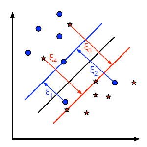
The red and blue lines that appear on the picture are the margins to each one of the decision regions. It is very important to realize that each of the \(\xi_{i}\) goes from a misclassified training sample to the margin of its appropriate region.

Finally, the new formulation for the optimization problem is:

\[\min_{\beta, \beta_{0}} L(\beta) = ||\beta||^{2} + C \sum_{i} {\xi_{i}} \text{ subject to } y_{i}(\beta^{T} x_{i} + \beta_{0}) \geq 1 - \xi_{i} \text{ and } \xi_{i} \geq 0 \text{ } \forall i\]

How should the parameter C be chosen? It is obvious that the answer to this question depends on how the training data is distributed. Although there is no general answer, it is useful to take into account these rules:

Source Code

You may also find the source code in samples/cpp/tutorial_code/ml/non_linear_svms folder of the OpenCV source library or download it from here.

Note
The following code has been implemented with OpenCV 3.0 classes and functions. An equivalent version of the code using OpenCV 2.4 can be found in this page.
#include <iostream>
#include <opencv2/core.hpp>
#include <opencv2/ml.hpp>
#define NTRAINING_SAMPLES 100 // Number of training samples per class
#define FRAC_LINEAR_SEP 0.9f // Fraction of samples which compose the linear separable part
using namespace cv;
using namespace cv::ml;
using namespace std;
static void help()
{
cout<< "\n--------------------------------------------------------------------------" << endl
<< "This program shows Support Vector Machines for Non-Linearly Separable Data. " << endl
<< "Usage:" << endl
<< "./non_linear_svms" << endl
<< "--------------------------------------------------------------------------" << endl
<< endl;
}
int main()
{
help();
// Data for visual representation
const int WIDTH = 512, HEIGHT = 512;
Mat I = Mat::zeros(HEIGHT, WIDTH, CV_8UC3);
//--------------------- 1. Set up training data randomly ---------------------------------------
Mat trainData(2*NTRAINING_SAMPLES, 2, CV_32FC1);
Mat labels (2*NTRAINING_SAMPLES, 1, CV_32SC1);
RNG rng(100); // Random value generation class
// Set up the linearly separable part of the training data
int nLinearSamples = (int) (FRAC_LINEAR_SEP * NTRAINING_SAMPLES);
// Generate random points for the class 1
Mat trainClass = trainData.rowRange(0, nLinearSamples);
// The x coordinate of the points is in [0, 0.4)
Mat c = trainClass.colRange(0, 1);
rng.fill(c, RNG::UNIFORM, Scalar(1), Scalar(0.4 * WIDTH));
// The y coordinate of the points is in [0, 1)
c = trainClass.colRange(1,2);
rng.fill(c, RNG::UNIFORM, Scalar(1), Scalar(HEIGHT));
// Generate random points for the class 2
trainClass = trainData.rowRange(2*NTRAINING_SAMPLES-nLinearSamples, 2*NTRAINING_SAMPLES);
// The x coordinate of the points is in [0.6, 1]
c = trainClass.colRange(0 , 1);
rng.fill(c, RNG::UNIFORM, Scalar(0.6*WIDTH), Scalar(WIDTH));
// The y coordinate of the points is in [0, 1)
c = trainClass.colRange(1,2);
rng.fill(c, RNG::UNIFORM, Scalar(1), Scalar(HEIGHT));
//------------------ Set up the non-linearly separable part of the training data ---------------
// Generate random points for the classes 1 and 2
trainClass = trainData.rowRange( nLinearSamples, 2*NTRAINING_SAMPLES-nLinearSamples);
// The x coordinate of the points is in [0.4, 0.6)
c = trainClass.colRange(0,1);
rng.fill(c, RNG::UNIFORM, Scalar(0.4*WIDTH), Scalar(0.6*WIDTH));
// The y coordinate of the points is in [0, 1)
c = trainClass.colRange(1,2);
rng.fill(c, RNG::UNIFORM, Scalar(1), Scalar(HEIGHT));
//------------------------- Set up the labels for the classes ---------------------------------
labels.rowRange( 0, NTRAINING_SAMPLES).setTo(1); // Class 1
labels.rowRange(NTRAINING_SAMPLES, 2*NTRAINING_SAMPLES).setTo(2); // Class 2
//------------------------ 2. Set up the support vector machines parameters --------------------
//------------------------ 3. Train the svm ----------------------------------------------------
cout << "Starting training process" << endl;
svm->setC(0.1);
svm->train(trainData, ROW_SAMPLE, labels);
cout << "Finished training process" << endl;
//------------------------ 4. Show the decision regions ----------------------------------------
Vec3b green(0,100,0), blue (100,0,0);
for (int i = 0; i < I.rows; ++i)
for (int j = 0; j < I.cols; ++j)
{
Mat sampleMat = (Mat_<float>(1,2) << i, j);
float response = svm->predict(sampleMat);
if (response == 1) I.at<Vec3b>(j, i) = green;
else if (response == 2) I.at<Vec3b>(j, i) = blue;
}
//----------------------- 5. Show the training data --------------------------------------------
int thick = -1;
int lineType = 8;
float px, py;
// Class 1
for (int i = 0; i < NTRAINING_SAMPLES; ++i)
{
px = trainData.at<float>(i,0);
py = trainData.at<float>(i,1);
circle(I, Point( (int) px, (int) py ), 3, Scalar(0, 255, 0), thick, lineType);
}
// Class 2
for (int i = NTRAINING_SAMPLES; i <2*NTRAINING_SAMPLES; ++i)
{
px = trainData.at<float>(i,0);
py = trainData.at<float>(i,1);
circle(I, Point( (int) px, (int) py ), 3, Scalar(255, 0, 0), thick, lineType);
}
//------------------------- 6. Show support vectors --------------------------------------------
thick = 2;
lineType = 8;
for (int i = 0; i < sv.rows; ++i)
{
const float* v = sv.ptr<float>(i);
circle( I, Point( (int) v[0], (int) v[1]), 6, Scalar(128, 128, 128), thick, lineType);
}
imwrite("result.png", I); // save the Image
imshow("SVM for Non-Linear Training Data", I); // show it to the user
waitKey(0);
}

Explanation

  1. Set up the training data

    The training data of this exercise is formed by a set of labeled 2D-points that belong to one of two different classes. To make the exercise more appealing, the training data is generated randomly using a uniform probability density functions (PDFs).

    We have divided the generation of the training data into two main parts.

    In the first part we generate data for both classes that is linearly separable.

    // Generate random points for the class 1
    Mat trainClass = trainData.rowRange(0, nLinearSamples);
    // The x coordinate of the points is in [0, 0.4)
    Mat c = trainClass.colRange(0, 1);
    rng.fill(c, RNG::UNIFORM, Scalar(1), Scalar(0.4 * WIDTH));
    // The y coordinate of the points is in [0, 1)
    c = trainClass.colRange(1,2);
    rng.fill(c, RNG::UNIFORM, Scalar(1), Scalar(HEIGHT));
    // Generate random points for the class 2
    trainClass = trainData.rowRange(2*NTRAINING_SAMPLES-nLinearSamples, 2*NTRAINING_SAMPLES);
    // The x coordinate of the points is in [0.6, 1]
    c = trainClass.colRange(0 , 1);
    rng.fill(c, RNG::UNIFORM, Scalar(0.6*WIDTH), Scalar(WIDTH));
    // The y coordinate of the points is in [0, 1)
    c = trainClass.colRange(1,2);
    rng.fill(c, RNG::UNIFORM, Scalar(1), Scalar(HEIGHT));

    In the second part we create data for both classes that is non-linearly separable, data that overlaps.

    // Generate random points for the classes 1 and 2
    trainClass = trainData.rowRange( nLinearSamples, 2*NTRAINING_SAMPLES-nLinearSamples);
    // The x coordinate of the points is in [0.4, 0.6)
    c = trainClass.colRange(0,1);
    rng.fill(c, RNG::UNIFORM, Scalar(0.4*WIDTH), Scalar(0.6*WIDTH));
    // The y coordinate of the points is in [0, 1)
    c = trainClass.colRange(1,2);
    rng.fill(c, RNG::UNIFORM, Scalar(1), Scalar(HEIGHT));
  2. Set up SVM's parameters

    Note
    In the previous tutorial Introduction to Support Vector Machines there is an explanation of the attributes of the class cv::ml::SVM that we configure here before training the SVM.
    Ptr<SVM> svm = SVM::create();
    svm->setType(SVM::C_SVC);
    svm->setC(0.1);
    svm->setKernel(SVM::LINEAR);
    svm->setTermCriteria(TermCriteria(TermCriteria::MAX_ITER, (int)1e7, 1e-6));

    There are just two differences between the configuration we do here and the one that was done in the previous tutorial (Introduction to Support Vector Machines) that we use as reference.

    • C. We chose here a small value of this parameter in order not to punish too much the misclassification errors in the optimization. The idea of doing this stems from the will of obtaining a solution close to the one intuitively expected. However, we recommend to get a better insight of the problem by making adjustments to this parameter.

      Note
      In this case there are just very few points in the overlapping region between classes. By giving a smaller value to FRAC_LINEAR_SEP the density of points can be incremented and the impact of the parameter C explored deeply.
    • Termination Criteria of the algorithm. The maximum number of iterations has to be increased considerably in order to solve correctly a problem with non-linearly separable training data. In particular, we have increased in five orders of magnitude this value.
  3. Train the SVM

    We call the method cv::ml::SVM::train to build the SVM model. Watch out that the training process may take a quite long time. Have patiance when your run the program.

    svm->train(trainData, ROW_SAMPLE, labels);
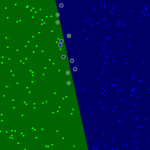
  4. Show the Decision Regions

    The method cv::ml::SVM::predict is used to classify an input sample using a trained SVM. In this example we have used this method in order to color the space depending on the prediction done by the SVM. In other words, an image is traversed interpreting its pixels as points of the Cartesian plane. Each of the points is colored depending on the class predicted by the SVM; in dark green if it is the class with label 1 and in dark blue if it is the class with label 2.

    Vec3b green(0,100,0), blue (100,0,0);
    for (int i = 0; i < I.rows; ++i)
    for (int j = 0; j < I.cols; ++j)
    {
    Mat sampleMat = (Mat_<float>(1,2) << i, j);
    float response = svm->predict(sampleMat);
    if (response == 1) I.at<Vec3b>(j, i) = green;
    else if (response == 2) I.at<Vec3b>(j, i) = blue;
    }
  5. Show the training data

    The method cv::circle is used to show the samples that compose the training data. The samples of the class labeled with 1 are shown in light green and in light blue the samples of the class labeled with 2.

    int thick = -1;
    int lineType = 8;
    float px, py;
    // Class 1
    for (int i = 0; i < NTRAINING_SAMPLES; ++i)
    {
    px = trainData.at<float>(i,0);
    py = trainData.at<float>(i,1);
    circle(I, Point( (int) px, (int) py ), 3, Scalar(0, 255, 0), thick, lineType);
    }
    // Class 2
    for (int i = NTRAINING_SAMPLES; i <2*NTRAINING_SAMPLES; ++i)
    {
    px = trainData.at<float>(i,0);
    py = trainData.at<float>(i,1);
    circle(I, Point( (int) px, (int) py ), 3, Scalar(255, 0, 0), thick, lineType);
    }
  6. Support vectors

    We use here a couple of methods to obtain information about the support vectors. The method cv::ml::SVM::getSupportVectors obtain all support vectors. We have used this methods here to find the training examples that are support vectors and highlight them.

    thick = 2;
    lineType = 8;
    Mat sv = svm->getUncompressedSupportVectors();
    for (int i = 0; i < sv.rows; ++i)
    {
    const float* v = sv.ptr<float>(i);
    circle( I, Point( (int) v[0], (int) v[1]), 6, Scalar(128, 128, 128), thick, lineType);
    }

    Results

svm_non_linear_result.png

You may observe a runtime instance of this on the YouTube here.