Disparity map post-filtering

Introduction

Stereo matching algorithms, especially highly-optimized ones that are intended for real-time processing on CPU, tend to make quite a few errors on challenging sequences. These errors are usually concentrated in uniform texture-less areas, half-occlusions and regions near depth discontinuities. One way of dealing with stereo-matching errors is to use various techniques of detecting potentially inaccurate disparity values and invalidate them, therefore making the disparity map semi-sparse. Several such techniques are already implemented in the StereoBM and StereoSGBM algorithms. Another way would be to use some kind of filtering procedure to align the disparity map edges with those of the source image and to propagate the disparity values from high- to low-confidence regions like half-occlusions. Recent advances in edge-aware filtering have enabled performing such post-filtering under the constraints of real-time processing on CPU.

In this tutorial you will learn how to use the disparity map post-filtering to improve the results of StereoBM and StereoSGBM algorithms.

Source Stereoscopic Image

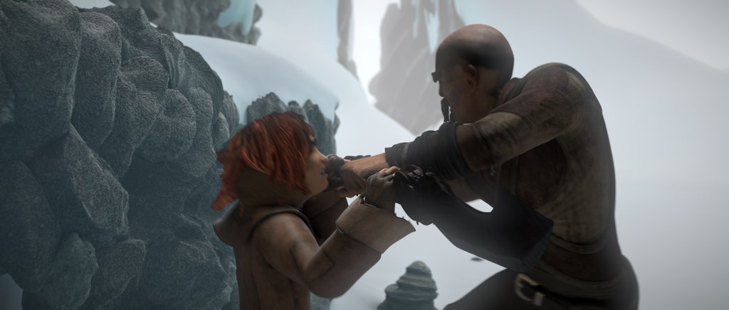
Left view

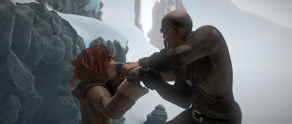
Right view

Source Code

We will be using snippets from the example application, that can be downloaded here.

Explanation

The provided example has several options that yield different trade-offs between the speed and the quality of the resulting disparity map. Both the speed and the quality are measured if the user has provided the ground-truth disparity map. In this tutorial we will take a detailed look at the default pipeline, that was designed to provide the best possible quality under the constraints of real-time processing on CPU.

1. Load left and right views

       Mat left  = imread(left_im ,IMREAD_COLOR);
       if ( left.empty() )
       {
           cout<<"Cannot read image file: "<<left_im;
           return -1;
       }
   
       Mat right = imread(right_im,IMREAD_COLOR);
       if ( right.empty() )
       {
           cout<<"Cannot read image file: "<<right_im;
           return -1;
       }

   We start by loading the source stereopair. For this tutorial we will take a somewhat challenging example from the MPI-Sintel dataset with a lot of texture-less regions.
2. Prepare the views for matching

               max_disp/=2;
               if(max_disp%16!=0)
                   max_disp += 16-(max_disp%16);
               resize(left ,left_for_matcher ,Size(),0.5,0.5, INTER_LINEAR_EXACT);
               resize(right,right_for_matcher,Size(),0.5,0.5, INTER_LINEAR_EXACT);

   We perform downscaling of the views to speed-up the matching stage at the cost of minor quality degradation. To get the best possible quality downscaling should be avoided.
3. Perform matching and create the filter instance

               Ptr<StereoBM> left_matcher = StereoBM::create(max_disp,wsize);
               wls_filter = createDisparityWLSFilter(left_matcher);
               Ptr<StereoMatcher> right_matcher = createRightMatcher(left_matcher);
   
               cvtColor(left_for_matcher,  left_for_matcher,  COLOR_BGR2GRAY);
               cvtColor(right_for_matcher, right_for_matcher, COLOR_BGR2GRAY);
   
               matching_time = (double)getTickCount();
               left_matcher-> compute(left_for_matcher, right_for_matcher,left_disp);
               right_matcher->compute(right_for_matcher,left_for_matcher, right_disp);
               matching_time = ((double)getTickCount() - matching_time)/getTickFrequency();

   We are using StereoBM for faster processing. If speed is not critical, though, StereoSGBM would provide better quality. The filter instance is created by providing the StereoMatcher instance that we intend to use. Another matcher instance is returned by the createRightMatcher function. These two matcher instances are then used to compute disparity maps both for the left and right views, that are required by the filter.
4. Perform filtering

           wls_filter->setLambda(lambda);
           wls_filter->setSigmaColor(sigma);
           filtering_time = (double)getTickCount();
           wls_filter->filter(left_disp,left,filtered_disp,right_disp);
           filtering_time = ((double)getTickCount() - filtering_time)/getTickFrequency();

   Disparity maps computed by the respective matcher instances, as well as the source left view are passed to the filter. Note that we are using the original non-downscaled view to guide the filtering process. The disparity map is automatically upscaled in an edge-aware fashion to match the original view resolution. The result is stored in filtered_disp.
5. Visualize the disparity maps

           Mat raw_disp_vis;
           getDisparityVis(left_disp,raw_disp_vis,vis_mult);
           namedWindow("raw disparity", WINDOW_AUTOSIZE);
           imshow("raw disparity", raw_disp_vis);
           Mat filtered_disp_vis;
           getDisparityVis(filtered_disp,filtered_disp_vis,vis_mult);
           namedWindow("filtered disparity", WINDOW_AUTOSIZE);
           imshow("filtered disparity", filtered_disp_vis);
           waitKey();

   We use a convenience function getDisparityVis to visualize the disparity maps. The second parameter defines the contrast (all disparity values are scaled by this value in the visualization).

Results

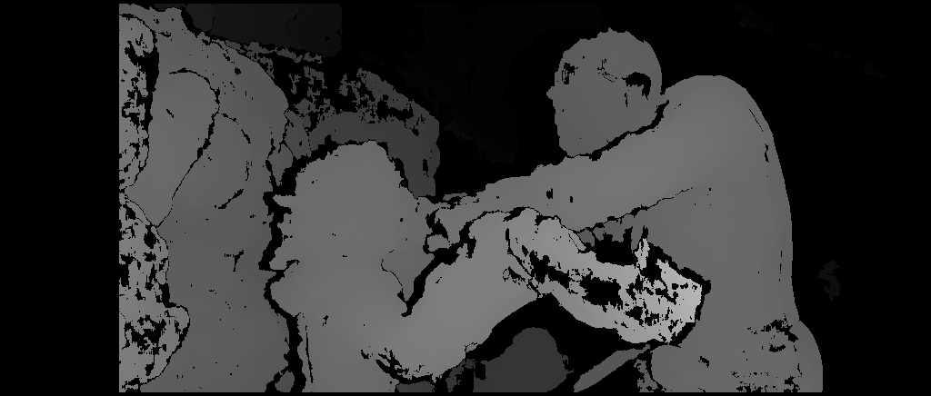
Result of the StereoBM

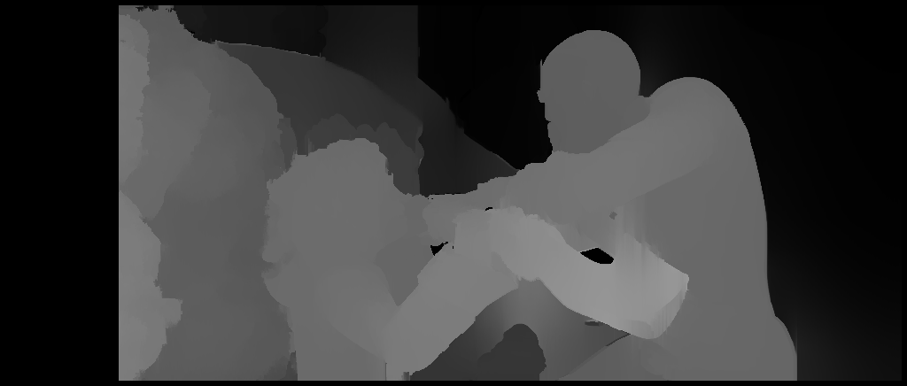
Result of the demonstrated pipeline (StereoBM on downscaled views with post-filtering)