Hough Line Transform

Prev Tutorial: Canny Edge Detector

Next Tutorial: Hough Circle Transform

Goal

In this tutorial you will learn how to:

• Use the OpenCV functions HoughLines() and HoughLinesP() to detect lines in an image.

Theory

Note

The explanation below belongs to the book Learning OpenCV by Bradski and Kaehler.

Hough Line Transform

1. The Hough Line Transform is a transform used to detect straight lines.
2. To apply the Transform, first an edge detection pre-processing is desirable.

How does it work?

1. As you know, a line in the image space can be expressed with two variables. For example:

   1. In the Cartesian coordinate system: Parameters: \((m,b)\).
   2. In the Polar coordinate system: Parameters: \((r,\theta)\)
   

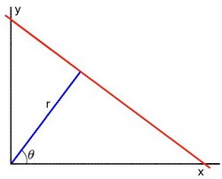
   For Hough Transforms, we will express lines in the Polar system. Hence, a line equation can be written as:

   \[y = \left ( -\dfrac{\cos \theta}{\sin \theta} \right ) x + \left ( \dfrac{r}{\sin \theta} \right )\]

Arranging the terms: \(r = x \cos \theta + y \sin \theta\)

1. In general for each point \((x_{0}, y_{0})\), we can define the family of lines that goes through that point as:

   \[r_{\theta} = x_{0} \cdot \cos \theta + y_{0} \cdot \sin \theta\]

   Meaning that each pair \((r_{\theta},\theta)\) represents each line that passes by \((x_{0}, y_{0})\).

2. If for a given \((x_{0}, y_{0})\) we plot the family of lines that goes through it, we get a sinusoid. For instance, for \(x_{0} = 8\) and \(y_{0} = 6\) we get the following plot (in a plane \(\theta\) - \(r\)):

   

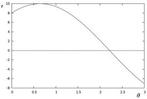
   We consider only points such that \(r > 0\) and \(0< \theta < 2 \pi\).

3. We can do the same operation above for all the points in an image. If the curves of two different points intersect in the plane \(\theta\) - \(r\), that means that both points belong to a same line. For instance, following with the example above and drawing the plot for two more points: \(x_{1} = 4\), \(y_{1} = 9\) and \(x_{2} = 12\), \(y_{2} = 3\), we get:

   

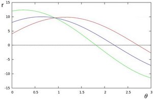
   The three plots intersect in one single point \((0.925, 9.6)\), these coordinates are the parameters ( \(\theta, r\)) or the line in which \((x_{0}, y_{0})\), \((x_{1}, y_{1})\) and \((x_{2}, y_{2})\) lay.

4. What does all the stuff above mean? It means that in general, a line can be detected by finding the number of intersections between curves.The more curves intersecting means that the line represented by that intersection have more points. In general, we can define a threshold of the minimum number of intersections needed to detect a line.
5. This is what the Hough Line Transform does. It keeps track of the intersection between curves of every point in the image. If the number of intersections is above some threshold, then it declares it as a line with the parameters \((\theta, r_{\theta})\) of the intersection point.

Standard and Probabilistic Hough Line Transform

OpenCV implements two kind of Hough Line Transforms:

a. The Standard Hough Transform

• It consists in pretty much what we just explained in the previous section. It gives you as result a vector of couples \((\theta, r_{\theta})\)
• In OpenCV it is implemented with the function HoughLines()

b. The Probabilistic Hough Line Transform

• A more efficient implementation of the Hough Line Transform. It gives as output the extremes of the detected lines \((x_{0}, y_{0}, x_{1}, y_{1})\)
• In OpenCV it is implemented with the function HoughLinesP()

What does this program do?

• Loads an image
• Applies a Standard Hough Line Transform and a Probabilistic Line Transform.
• Display the original image and the detected line in three windows.

Code

C++

The sample code that we will explain can be downloaded from here. A slightly fancier version (which shows both Hough standard and probabilistic with trackbars for changing the threshold values) can be found here.

#include "opencv2/imgcodecs.hpp"
#include "opencv2/highgui.hpp"
#include "opencv2/imgproc.hpp"

using namespace cv;
using namespace std;

int main(int argc, char** argv)
{
    // Declare the output variables
    Mat dst, cdst, cdstP;

    const char* default_file = "../../../data/sudoku.png";
    const char* filename = argc >=2 ? argv[1] : default_file;

    // Loads an image
    Mat src = imread( filename, IMREAD_GRAYSCALE );

    // Check if image is loaded fine
    if(src.empty()){
        printf(" Error opening image\n");
        printf(" Program Arguments: [image_name -- default %s] \n", default_file);
        return -1;
    }

    // Edge detection
    Canny(src, dst, 50, 200, 3);

    // Copy edges to the images that will display the results in BGR
    cvtColor(dst, cdst, COLOR_GRAY2BGR);
    cdstP = cdst.clone();

    // Standard Hough Line Transform
    vector<Vec2f> lines; // will hold the results of the detection
    HoughLines(dst, lines, 1, CV_PI/180, 150, 0, 0 ); // runs the actual detection
    // Draw the lines
    for( size_t i = 0; i < lines.size(); i++ )
    {
        float rho = lines[i][0], theta = lines[i][1];
        Point pt1, pt2;
        double a = cos(theta), b = sin(theta);
        double x0 = a*rho, y0 = b*rho;
        pt1.x = cvRound(x0 + 1000*(-b));
        pt1.y = cvRound(y0 + 1000*(a));
        pt2.x = cvRound(x0 - 1000*(-b));
        pt2.y = cvRound(y0 - 1000*(a));
        line( cdst, pt1, pt2, Scalar(0,0,255), 3, CV_AA);
    }

    // Probabilistic Line Transform
    vector<Vec4i> linesP; // will hold the results of the detection
    HoughLinesP(dst, linesP, 1, CV_PI/180, 50, 50, 10 ); // runs the actual detection
    // Draw the lines
    for( size_t i = 0; i < linesP.size(); i++ )
    {
        Vec4i l = linesP[i];
        line( cdstP, Point(l[0], l[1]), Point(l[2], l[3]), Scalar(0,0,255), 3, LINE_AA);
    }

    // Show results
    imshow("Source", src);
    imshow("Detected Lines (in red) - Standard Hough Line Transform", cdst);
    imshow("Detected Lines (in red) - Probabilistic Line Transform", cdstP);

    // Wait and Exit
    waitKey();
    return 0;
}

Java

The sample code that we will explain can be downloaded from here.

import org.opencv.core.*;
import org.opencv.core.Point;
import org.opencv.highgui.HighGui;
import org.opencv.imgcodecs.Imgcodecs;
import org.opencv.imgproc.Imgproc;

class HoughLinesRun {

    public void run(String[] args) {
        // Declare the output variables
        Mat dst = new Mat(), cdst = new Mat(), cdstP;

        String default_file = "../../../../data/sudoku.png";
        String filename = ((args.length > 0) ? args[0] : default_file);

        // Load an image
        Mat src = Imgcodecs.imread(filename, Imgcodecs.IMREAD_GRAYSCALE);

        // Check if image is loaded fine
        if( src.empty() ) {
            System.out.println("Error opening image!");
            System.out.println("Program Arguments: [image_name -- default "
                    + default_file +"] \n");
            System.exit(-1);
        }

        // Edge detection
        Imgproc.Canny(src, dst, 50, 200, 3, false);

        // Copy edges to the images that will display the results in BGR
        Imgproc.cvtColor(dst, cdst, Imgproc.COLOR_GRAY2BGR);
        cdstP = cdst.clone();

        // Standard Hough Line Transform
        Mat lines = new Mat(); // will hold the results of the detection
        Imgproc.HoughLines(dst, lines, 1, Math.PI/180, 150); // runs the actual detection
        // Draw the lines
        for (int x = 0; x < lines.rows(); x++) {
            double rho = lines.get(x, 0)[0],
                    theta = lines.get(x, 0)[1];

            double a = Math.cos(theta), b = Math.sin(theta);
            double x0 = a*rho, y0 = b*rho;
            Point pt1 = new Point(Math.round(x0 + 1000*(-b)), Math.round(y0 + 1000*(a)));
            Point pt2 = new Point(Math.round(x0 - 1000*(-b)), Math.round(y0 - 1000*(a)));
            Imgproc.line(cdst, pt1, pt2, new Scalar(0, 0, 255), 3, Imgproc.LINE_AA, 0);
        }

        // Probabilistic Line Transform
        Mat linesP = new Mat(); // will hold the results of the detection
        Imgproc.HoughLinesP(dst, linesP, 1, Math.PI/180, 50, 50, 10); // runs the actual detection
        // Draw the lines
        for (int x = 0; x < linesP.rows(); x++) {
            double[] l = linesP.get(x, 0);
            Imgproc.line(cdstP, new Point(l[0], l[1]), new Point(l[2], l[3]), new Scalar(0, 0, 255), 3, Imgproc.LINE_AA, 0);
        }

        // Show results
        HighGui.imshow("Source", src);
        HighGui.imshow("Detected Lines (in red) - Standard Hough Line Transform", cdst);
        HighGui.imshow("Detected Lines (in red) - Probabilistic Line Transform", cdstP);

        // Wait and Exit
        HighGui.waitKey();
        System.exit(0);
    }
}

public class HoughLines {
    public static void main(String[] args) {
        // Load the native library.
        System.loadLibrary(Core.NATIVE_LIBRARY_NAME);
        new HoughLinesRun().run(args);
    }
}

Python

The sample code that we will explain can be downloaded from here.

"""
@file hough_lines.py
@brief This program demonstrates line finding with the Hough transform
"""
import sys
import math
import cv2
import numpy as np


def main(argv):
    
    default_file =  "../../../../data/sudoku.png"
    filename = argv[0] if len(argv) > 0 else default_file

    # Loads an image
    src = cv2.imread(filename, cv2.IMREAD_GRAYSCALE)

    # Check if image is loaded fine
    if src is None:
        print ('Error opening image!')
        print ('Usage: hough_lines.py [image_name -- default ' + default_file + '] \n')
        return -1
    

    
    dst = cv2.Canny(src, 50, 200, None, 3)
    

    # Copy edges to the images that will display the results in BGR
    cdst = cv2.cvtColor(dst, cv2.COLOR_GRAY2BGR)
    cdstP = np.copy(cdst)

    
    lines = cv2.HoughLines(dst, 1, np.pi / 180, 150, None, 0, 0)
    
    if lines is not None:
        for i in range(0, len(lines)):
            rho = lines[i][0][0]
            theta = lines[i][0][1]
            a = math.cos(theta)
            b = math.sin(theta)
            x0 = a * rho
            y0 = b * rho
            pt1 = (int(x0 + 1000*(-b)), int(y0 + 1000*(a)))
            pt2 = (int(x0 - 1000*(-b)), int(y0 - 1000*(a)))

            cv2.line(cdst, pt1, pt2, (0,0,255), 3, cv2.LINE_AA)
    

    
    linesP = cv2.HoughLinesP(dst, 1, np.pi / 180, 50, None, 50, 10)
    
    if linesP is not None:
        for i in range(0, len(linesP)):
            l = linesP[i][0]
            cv2.line(cdstP, (l[0], l[1]), (l[2], l[3]), (0,0,255), 3, cv2.LINE_AA)
    
    cv2.imshow("Source", src)
    cv2.imshow("Detected Lines (in red) - Standard Hough Line Transform", cdst)
    cv2.imshow("Detected Lines (in red) - Probabilistic Line Transform", cdstP)
    
    cv2.waitKey()
    return 0
    

if __name__ == "__main__":
    main(sys.argv[1:])

Explanation

Load an image:

C++

    const char* default_file = "../../../data/sudoku.png";
    const char* filename = argc >=2 ? argv[1] : default_file;

    // Loads an image
    Mat src = imread( filename, IMREAD_GRAYSCALE );

    // Check if image is loaded fine
    if(src.empty()){
        printf(" Error opening image\n");
        printf(" Program Arguments: [image_name -- default %s] \n", default_file);
        return -1;
    }

Java

        String default_file = "../../../../data/sudoku.png";
        String filename = ((args.length > 0) ? args[0] : default_file);

        // Load an image
        Mat src = Imgcodecs.imread(filename, Imgcodecs.IMREAD_GRAYSCALE);

        // Check if image is loaded fine
        if( src.empty() ) {
            System.out.println("Error opening image!");
            System.out.println("Program Arguments: [image_name -- default "
                    + default_file +"] \n");
            System.exit(-1);
        }

Python

    default_file =  "../../../../data/sudoku.png"
    filename = argv[0] if len(argv) > 0 else default_file

    # Loads an image
    src = cv2.imread(filename, cv2.IMREAD_GRAYSCALE)

    # Check if image is loaded fine
    if src is None:
        print ('Error opening image!')
        print ('Usage: hough_lines.py [image_name -- default ' + default_file + '] \n')
        return -1

Detect the edges of the image by using a Canny detector:

C++

    // Edge detection
    Canny(src, dst, 50, 200, 3);

Java

        // Edge detection
        Imgproc.Canny(src, dst, 50, 200, 3, false);

Python

    # Edge detection
    dst = cv2.Canny(src, 50, 200, None, 3)

Now we will apply the Hough Line Transform. We will explain how to use both OpenCV functions available for this purpose.

Standard Hough Line Transform:

First, you apply the Transform:

C++

    // Standard Hough Line Transform
    vector<Vec2f> lines; // will hold the results of the detection
    HoughLines(dst, lines, 1, CV_PI/180, 150, 0, 0 ); // runs the actual detection

Java

        // Standard Hough Line Transform
        Mat lines = new Mat(); // will hold the results of the detection
        Imgproc.HoughLines(dst, lines, 1, Math.PI/180, 150); // runs the actual detection

Python

    #  Standard Hough Line Transform
    lines = cv2.HoughLines(dst, 1, np.pi / 180, 150, None, 0, 0)

• with the following arguments:
  • dst: Output of the edge detector. It should be a grayscale image (although in fact it is a binary one)
  • lines: A vector that will store the parameters \((r,\theta)\) of the detected lines
  • rho : The resolution of the parameter \(r\) in pixels. We use 1 pixel.
  • theta: The resolution of the parameter \(\theta\) in radians. We use 1 degree (CV_PI/180)
  • threshold: The minimum number of intersections to "*detect*" a line
  • srn and stn: Default parameters to zero. Check OpenCV reference for more info.

And then you display the result by drawing the lines.

C++

    // Draw the lines
    for( size_t i = 0; i < lines.size(); i++ )
    {
        float rho = lines[i][0], theta = lines[i][1];
        Point pt1, pt2;
        double a = cos(theta), b = sin(theta);
        double x0 = a*rho, y0 = b*rho;
        pt1.x = cvRound(x0 + 1000*(-b));
        pt1.y = cvRound(y0 + 1000*(a));
        pt2.x = cvRound(x0 - 1000*(-b));
        pt2.y = cvRound(y0 - 1000*(a));
        line( cdst, pt1, pt2, Scalar(0,0,255), 3, CV_AA);
    }

Java

        // Draw the lines
        for (int x = 0; x < lines.rows(); x++) {
            double rho = lines.get(x, 0)[0],
                    theta = lines.get(x, 0)[1];

            double a = Math.cos(theta), b = Math.sin(theta);
            double x0 = a*rho, y0 = b*rho;
            Point pt1 = new Point(Math.round(x0 + 1000*(-b)), Math.round(y0 + 1000*(a)));
            Point pt2 = new Point(Math.round(x0 - 1000*(-b)), Math.round(y0 - 1000*(a)));
            Imgproc.line(cdst, pt1, pt2, new Scalar(0, 0, 255), 3, Imgproc.LINE_AA, 0);
        }

Python

    # Draw the lines
    if lines is not None:
        for i in range(0, len(lines)):
            rho = lines[i][0][0]
            theta = lines[i][0][1]
            a = math.cos(theta)
            b = math.sin(theta)
            x0 = a * rho
            y0 = b * rho
            pt1 = (int(x0 + 1000*(-b)), int(y0 + 1000*(a)))
            pt2 = (int(x0 - 1000*(-b)), int(y0 - 1000*(a)))

            cv2.line(cdst, pt1, pt2, (0,0,255), 3, cv2.LINE_AA)

Probabilistic Hough Line Transform

First you apply the transform:

C++

    // Probabilistic Line Transform
    vector<Vec4i> linesP; // will hold the results of the detection
    HoughLinesP(dst, linesP, 1, CV_PI/180, 50, 50, 10 ); // runs the actual detection

Java

        // Probabilistic Line Transform
        Mat linesP = new Mat(); // will hold the results of the detection
        Imgproc.HoughLinesP(dst, linesP, 1, Math.PI/180, 50, 50, 10); // runs the actual detection

Python

    # Probabilistic Line Transform
    linesP = cv2.HoughLinesP(dst, 1, np.pi / 180, 50, None, 50, 10)

• with the arguments:
  • dst: Output of the edge detector. It should be a grayscale image (although in fact it is a binary one)
  • lines: A vector that will store the parameters \((x_{start}, y_{start}, x_{end}, y_{end})\) of the detected lines
  • rho : The resolution of the parameter \(r\) in pixels. We use 1 pixel.
  • theta: The resolution of the parameter \(\theta\) in radians. We use 1 degree (CV_PI/180)
  • threshold: The minimum number of intersections to "*detect*" a line
  • minLinLength: The minimum number of points that can form a line. Lines with less than this number of points are disregarded.
  • maxLineGap: The maximum gap between two points to be considered in the same line.

And then you display the result by drawing the lines.

C++

    // Draw the lines
    for( size_t i = 0; i < linesP.size(); i++ )
    {
        Vec4i l = linesP[i];
        line( cdstP, Point(l[0], l[1]), Point(l[2], l[3]), Scalar(0,0,255), 3, LINE_AA);
    }

Java

        // Draw the lines
        for (int x = 0; x < linesP.rows(); x++) {
            double[] l = linesP.get(x, 0);
            Imgproc.line(cdstP, new Point(l[0], l[1]), new Point(l[2], l[3]), new Scalar(0, 0, 255), 3, Imgproc.LINE_AA, 0);
        }

Python

    # Draw the lines
    if linesP is not None:
        for i in range(0, len(linesP)):
            l = linesP[i][0]
            cv2.line(cdstP, (l[0], l[1]), (l[2], l[3]), (0,0,255), 3, cv2.LINE_AA)

Display the original image and the detected lines:

C++

    // Show results
    imshow("Source", src);
    imshow("Detected Lines (in red) - Standard Hough Line Transform", cdst);
    imshow("Detected Lines (in red) - Probabilistic Line Transform", cdstP);

Java

        // Show results
        HighGui.imshow("Source", src);
        HighGui.imshow("Detected Lines (in red) - Standard Hough Line Transform", cdst);
        HighGui.imshow("Detected Lines (in red) - Probabilistic Line Transform", cdstP);

Python

    # Show results
    cv2.imshow("Source", src)
    cv2.imshow("Detected Lines (in red) - Standard Hough Line Transform", cdst)
    cv2.imshow("Detected Lines (in red) - Probabilistic Line Transform", cdstP)

Wait until the user exits the program

C++

    // Wait and Exit
    waitKey();
    return 0;

Java

        // Wait and Exit
        HighGui.waitKey();
        System.exit(0);

Python

    # Wait and Exit
    cv2.waitKey()
    return 0

Result

Note

The results below are obtained using the slightly fancier version we mentioned in the Code section. It still implements the same stuff as above, only adding the Trackbar for the Threshold.

Using an input image such as a sudoku image. We get the following result by using the Standard Hough Line Transform:

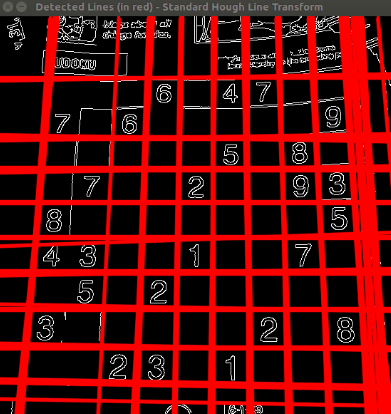
And by using the Probabilistic Hough Line Transform:

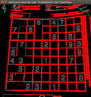
You may observe that the number of lines detected vary while you change the threshold. The explanation is sort of evident: If you establish a higher threshold, fewer lines will be detected (since you will need more points to declare a line detected).