OpenCV  3.3.1
Open Source Computer Vision
Image Segmentation with Distance Transform and Watershed Algorithm

Goal

In this tutorial you will learn how to:

Theory

Code

This tutorial code's is shown lines below. You can also download it from here.

#include <opencv2/opencv.hpp>
#include <iostream>
using namespace std;
using namespace cv;
int main()
{
// Load the image
Mat src = imread("../data/cards.png");
// Check if everything was fine
if (!src.data)
return -1;
// Show source image
imshow("Source Image", src);
// Change the background from white to black, since that will help later to extract
// better results during the use of Distance Transform
for( int x = 0; x < src.rows; x++ ) {
for( int y = 0; y < src.cols; y++ ) {
if ( src.at<Vec3b>(x, y) == Vec3b(255,255,255) ) {
src.at<Vec3b>(x, y)[0] = 0;
src.at<Vec3b>(x, y)[1] = 0;
src.at<Vec3b>(x, y)[2] = 0;
}
}
}
// Show output image
imshow("Black Background Image", src);
// Create a kernel that we will use for accuting/sharpening our image
Mat kernel = (Mat_<float>(3,3) <<
1, 1, 1,
1, -8, 1,
1, 1, 1); // an approximation of second derivative, a quite strong kernel
// do the laplacian filtering as it is
// well, we need to convert everything in something more deeper then CV_8U
// because the kernel has some negative values,
// and we can expect in general to have a Laplacian image with negative values
// BUT a 8bits unsigned int (the one we are working with) can contain values from 0 to 255
// so the possible negative number will be truncated
Mat imgLaplacian;
Mat sharp = src; // copy source image to another temporary one
filter2D(sharp, imgLaplacian, CV_32F, kernel);
src.convertTo(sharp, CV_32F);
Mat imgResult = sharp - imgLaplacian;
// convert back to 8bits gray scale
imgResult.convertTo(imgResult, CV_8UC3);
imgLaplacian.convertTo(imgLaplacian, CV_8UC3);
// imshow( "Laplace Filtered Image", imgLaplacian );
imshow( "New Sharped Image", imgResult );
src = imgResult; // copy back
// Create binary image from source image
Mat bw;
cvtColor(src, bw, CV_BGR2GRAY);
imshow("Binary Image", bw);
// Perform the distance transform algorithm
Mat dist;
// Normalize the distance image for range = {0.0, 1.0}
// so we can visualize and threshold it
normalize(dist, dist, 0, 1., NORM_MINMAX);
imshow("Distance Transform Image", dist);
// Threshold to obtain the peaks
// This will be the markers for the foreground objects
threshold(dist, dist, .4, 1., CV_THRESH_BINARY);
// Dilate a bit the dist image
Mat kernel1 = Mat::ones(3, 3, CV_8UC1);
dilate(dist, dist, kernel1);
imshow("Peaks", dist);
// Create the CV_8U version of the distance image
// It is needed for findContours()
Mat dist_8u;
dist.convertTo(dist_8u, CV_8U);
// Find total markers
vector<vector<Point> > contours;
// Create the marker image for the watershed algorithm
Mat markers = Mat::zeros(dist.size(), CV_32SC1);
// Draw the foreground markers
for (size_t i = 0; i < contours.size(); i++)
drawContours(markers, contours, static_cast<int>(i), Scalar::all(static_cast<int>(i)+1), -1);
// Draw the background marker
circle(markers, Point(5,5), 3, CV_RGB(255,255,255), -1);
imshow("Markers", markers*10000);
// Perform the watershed algorithm
watershed(src, markers);
Mat mark = Mat::zeros(markers.size(), CV_8UC1);
markers.convertTo(mark, CV_8UC1);
bitwise_not(mark, mark);
// imshow("Markers_v2", mark); // uncomment this if you want to see how the mark
// image looks like at that point
// Generate random colors
vector<Vec3b> colors;
for (size_t i = 0; i < contours.size(); i++)
{
int b = theRNG().uniform(0, 255);
int g = theRNG().uniform(0, 255);
int r = theRNG().uniform(0, 255);
colors.push_back(Vec3b((uchar)b, (uchar)g, (uchar)r));
}
// Create the result image
Mat dst = Mat::zeros(markers.size(), CV_8UC3);
// Fill labeled objects with random colors
for (int i = 0; i < markers.rows; i++)
{
for (int j = 0; j < markers.cols; j++)
{
int index = markers.at<int>(i,j);
if (index > 0 && index <= static_cast<int>(contours.size()))
dst.at<Vec3b>(i,j) = colors[index-1];
else
dst.at<Vec3b>(i,j) = Vec3b(0,0,0);
}
}
// Visualize the final image
imshow("Final Result", dst);
waitKey(0);
return 0;
}

Explanation / Result

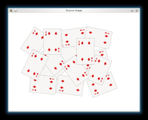
  1. Load the source image and check if it is loaded without any problem, then show it:
    // Load the image
    Mat src = imread("../data/cards.png");
    // Check if everything was fine
    if (!src.data)
    return -1;
    // Show source image
    imshow("Source Image", src);
    source.jpeg
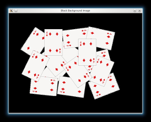
  2. Then if we have an image with white background, it is good to tranform it black. This will help us to desciminate the foreground objects easier when we will apply the Distance Transform:
    // Change the background from white to black, since that will help later to extract
    // better results during the use of Distance Transform
    for( int x = 0; x < src.rows; x++ ) {
    for( int y = 0; y < src.cols; y++ ) {
    if ( src.at<Vec3b>(x, y) == Vec3b(255,255,255) ) {
    src.at<Vec3b>(x, y)[0] = 0;
    src.at<Vec3b>(x, y)[1] = 0;
    src.at<Vec3b>(x, y)[2] = 0;
    }
    }
    }
    // Show output image
    imshow("Black Background Image", src);
    black_bg.jpeg
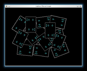
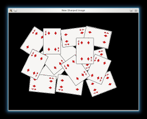
  3. Afterwards we will sharp our image in order to acute the edges of the foreground objects. We will apply a laplacian filter with a quite strong filter (an approximation of second derivative):
    // Create a kernel that we will use for accuting/sharpening our image
    Mat kernel = (Mat_<float>(3,3) <<
    1, 1, 1,
    1, -8, 1,
    1, 1, 1); // an approximation of second derivative, a quite strong kernel
    // do the laplacian filtering as it is
    // well, we need to convert everything in something more deeper then CV_8U
    // because the kernel has some negative values,
    // and we can expect in general to have a Laplacian image with negative values
    // BUT a 8bits unsigned int (the one we are working with) can contain values from 0 to 255
    // so the possible negative number will be truncated
    Mat imgLaplacian;
    Mat sharp = src; // copy source image to another temporary one
    filter2D(sharp, imgLaplacian, CV_32F, kernel);
    src.convertTo(sharp, CV_32F);
    Mat imgResult = sharp - imgLaplacian;
    // convert back to 8bits gray scale
    imgResult.convertTo(imgResult, CV_8UC3);
    imgLaplacian.convertTo(imgLaplacian, CV_8UC3);
    // imshow( "Laplace Filtered Image", imgLaplacian );
    imshow( "New Sharped Image", imgResult );
    laplace.jpeg
    sharp.jpeg
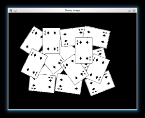
  4. Now we tranfrom our new sharped source image to a grayscale and a binary one, respectively:
    // Create binary image from source image
    Mat bw;
    cvtColor(src, bw, CV_BGR2GRAY);
    imshow("Binary Image", bw);
    bin.jpeg
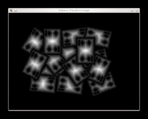
  5. We are ready now to apply the Distance Tranform on the binary image. Moreover, we normalize the output image in order to be able visualize and threshold the result:
    // Perform the distance transform algorithm
    Mat dist;
    // Normalize the distance image for range = {0.0, 1.0}
    // so we can visualize and threshold it
    normalize(dist, dist, 0, 1., NORM_MINMAX);
    imshow("Distance Transform Image", dist);
    dist_transf.jpeg
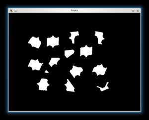
  6. We threshold the dist image and then perform some morphology operation (i.e. dilation) in order to extract the peaks from the above image:
    // Threshold to obtain the peaks
    // This will be the markers for the foreground objects
    threshold(dist, dist, .4, 1., CV_THRESH_BINARY);
    // Dilate a bit the dist image
    Mat kernel1 = Mat::ones(3, 3, CV_8UC1);
    dilate(dist, dist, kernel1);
    imshow("Peaks", dist);
    peaks.jpeg
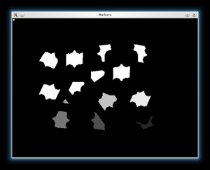
  7. From each blob then we create a seed/marker for the watershed algorithm with the help of the cv::findContours function:
    // Create the CV_8U version of the distance image
    // It is needed for findContours()
    Mat dist_8u;
    dist.convertTo(dist_8u, CV_8U);
    // Find total markers
    vector<vector<Point> > contours;
    // Create the marker image for the watershed algorithm
    Mat markers = Mat::zeros(dist.size(), CV_32SC1);
    // Draw the foreground markers
    for (size_t i = 0; i < contours.size(); i++)
    drawContours(markers, contours, static_cast<int>(i), Scalar::all(static_cast<int>(i)+1), -1);
    // Draw the background marker
    circle(markers, Point(5,5), 3, CV_RGB(255,255,255), -1);
    imshow("Markers", markers*10000);
    markers.jpeg
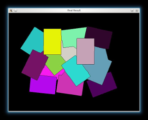
  8. Finally, we can apply the watershed algorithm, and visualize the result:
    // Perform the watershed algorithm
    watershed(src, markers);
    Mat mark = Mat::zeros(markers.size(), CV_8UC1);
    markers.convertTo(mark, CV_8UC1);
    bitwise_not(mark, mark);
    // imshow("Markers_v2", mark); // uncomment this if you want to see how the mark
    // image looks like at that point
    // Generate random colors
    vector<Vec3b> colors;
    for (size_t i = 0; i < contours.size(); i++)
    {
    int b = theRNG().uniform(0, 255);
    int g = theRNG().uniform(0, 255);
    int r = theRNG().uniform(0, 255);
    colors.push_back(Vec3b((uchar)b, (uchar)g, (uchar)r));
    }
    // Create the result image
    Mat dst = Mat::zeros(markers.size(), CV_8UC3);
    // Fill labeled objects with random colors
    for (int i = 0; i < markers.rows; i++)
    {
    for (int j = 0; j < markers.cols; j++)
    {
    int index = markers.at<int>(i,j);
    if (index > 0 && index <= static_cast<int>(contours.size()))
    dst.at<Vec3b>(i,j) = colors[index-1];
    else
    dst.at<Vec3b>(i,j) = Vec3b(0,0,0);
    }
    }
    // Visualize the final image
    imshow("Final Result", dst);
    final.jpeg