|
OpenCV
Open Source Computer Vision
|


•All Classes Namespaces Files Functions Variables Typedefs Enumerations Enumerator Properties Friends Macros Modules Pages
|
OpenCV
Open Source Computer Vision
|
In this tutorial you will learn how to apply diverse linear filters to smooth images using OpenCV functions such as:
To perform a smoothing operation we will apply a filter to our image. The most common type of filters are linear, in which an output pixel's value (i.e. g(i,j)) is determined as a weighted sum of input pixel values (i.e. f(i+k,j+l)) :
g(i,j) = \sum_{k,l} f(i+k, j+l) h(k,l)
h(k,l) is called the kernel, which is nothing more than the coefficients of the filter.
It helps to visualize a filter as a window of coefficients sliding across the image.
The kernel is below:
K = \dfrac{1}{K_{width} \cdot K_{height}} \begin{bmatrix} 1 & 1 & 1 & ... & 1 \\ 1 & 1 & 1 & ... & 1 \\ . & . & . & ... & 1 \\ . & . & . & ... & 1 \\ 1 & 1 & 1 & ... & 1 \end{bmatrix}
Just to make the picture clearer, remember how a 1D Gaussian kernel look like?
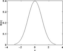
Assuming that an image is 1D, you can notice that the pixel located in the middle would have the biggest weight. The weight of its neighbors decreases as the spatial distance between them and the center pixel increases.
G_{0}(x, y) = A e^{ \dfrac{ -(x - \mu_{x})^{2} }{ 2\sigma^{2}_{x} } + \dfrac{ -(y - \mu_{y})^{2} }{ 2\sigma^{2}_{y} } }
The median filter run through each element of the signal (in this case the image) and replace each pixel with the median of its neighboring pixels (located in a square neighborhood around the evaluated pixel).
Normalized Block Filter:
OpenCV offers the function cv::blur to perform smoothing with this filter.
We specify 4 arguments (more details, check the Reference):
Gaussian Filter:
It is performed by the function cv::GaussianBlur :
Here we use 4 arguments (more details, check the OpenCV reference):
Median Filter:
This filter is provided by the cv::medianBlur function:
We use three arguments:
Bilateral Filter
Provided by OpenCV function cv::bilateralFilter
We use 5 arguments:
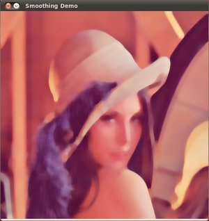
Here is a snapshot of the image smoothed using medianBlur:
 1.8.12