 |
OpenCV
3.4.2
Open Source Computer Vision
|
 |
OpenCV
3.4.2
Open Source Computer Vision
|
Prev Tutorial: Adding borders to your images
Next Tutorial: Laplace Operator
In this tutorial you will learn how to:
Why may be important the calculus of the derivatives in an image? Let's imagine we want to detect the edges present in the image. For instance:

You can easily notice that in an edge, the pixel intensity changes in a notorious way. A good way to express changes is by using derivatives. A high change in gradient indicates a major change in the image.
To be more graphical, let's assume we have a 1D-image. An edge is shown by the "jump" in intensity in the plot below:

The edge "jump" can be seen more easily if we take the first derivative (actually, here appears as a maximum)

Assuming that the image to be operated is \(I\):
We calculate two derivatives:
\[G_{x} = \begin{bmatrix} -1 & 0 & +1 \\ -2 & 0 & +2 \\ -1 & 0 & +1 \end{bmatrix} * I\]
\[G_{y} = \begin{bmatrix} -1 & -2 & -1 \\ 0 & 0 & 0 \\ +1 & +2 & +1 \end{bmatrix} * I\]
At each point of the image we calculate an approximation of the gradient in that point by combining both results above:
\[G = \sqrt{ G_{x}^{2} + G_{y}^{2} }\]
Although sometimes the following simpler equation is used:
\[G = |G_{x}| + |G_{y}|\]
3, the Sobel kernel shown above may produce noticeable inaccuracies (after all, Sobel is only an approximation of the derivative). OpenCV addresses this inaccuracy for kernels of size 3 by using the Scharr() function. This is as fast but more accurate than the standard Sobel function. It implements the following kernels: \[G_{x} = \begin{bmatrix} -3 & 0 & +3 \\ -10 & 0 & +10 \\ -3 & 0 & +3 \end{bmatrix}\]
\[G_{y} = \begin{bmatrix} -3 & -10 & -3 \\ 0 & 0 & 0 \\ +3 & +10 & +3 \end{bmatrix}\]
We calculate the "derivatives" in x and y directions. For this, we use the function Sobel() as shown below: The function takes the following arguments:
Notice that to calculate the gradient in x direction we use: \(x_{order}= 1\) and \(y_{order} = 0\). We do analogously for the y direction.
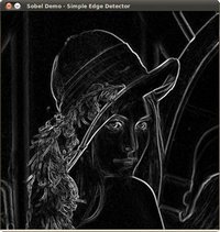
We try to approximate the gradient by adding both directional gradients (note that this is not an exact calculation at all! but it is good for our purposes).
Here is the output of applying our basic detector to lena.jpg:

 1.8.12