|
OpenCV
3.0.0
Open Source Computer Vision
|


All Classes Namespaces Files Functions Variables Typedefs Enumerations Enumerator Properties Friends Macros Groups Pages
|
OpenCV
3.0.0
Open Source Computer Vision
|
In this tutorial you will learn how to:
A Support Vector Machine (SVM) is a discriminative classifier formally defined by a separating hyperplane. In other words, given labeled training data (supervised learning), the algorithm outputs an optimal hyperplane which categorizes new examples.
In which sense is the hyperplane obtained optimal? Let's consider the following simple problem:
For a linearly separable set of 2D-points which belong to one of two classes, find a separating straight line.
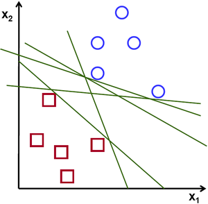
In the above picture you can see that there exists multiple lines that offer a solution to the problem. Is any of them better than the others? We can intuitively define a criterion to estimate the worth of the lines: A line is bad if it passes too close to the points because it will be noise sensitive and it will not generalize correctly. Therefore, our goal should be to find the line passing as far as possible from all points.
Then, the operation of the SVM algorithm is based on finding the hyperplane that gives the largest minimum distance to the training examples. Twice, this distance receives the important name of margin within SVM's theory. Therefore, the optimal separating hyperplane maximizes the margin of the training data.
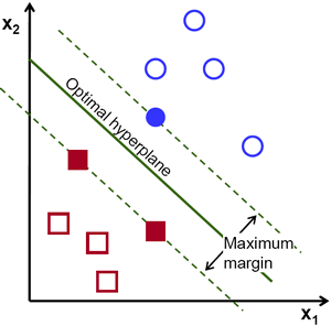
Let's introduce the notation used to define formally a hyperplane:
\[f(x) = \beta_{0} + \beta^{T} x,\]
where \(\beta\) is known as the weight vector and \(\beta_{0}\) as the bias.
The optimal hyperplane can be represented in an infinite number of different ways by scaling of \(\beta\) and \(\beta_{0}\). As a matter of convention, among all the possible representations of the hyperplane, the one chosen is
\[|\beta_{0} + \beta^{T} x| = 1\]
where \(x\) symbolizes the training examples closest to the hyperplane. In general, the training examples that are closest to the hyperplane are called support vectors. This representation is known as the canonical hyperplane.
Now, we use the result of geometry that gives the distance between a point \(x\) and a hyperplane \((\beta, \beta_{0})\):
\[\mathrm{distance} = \frac{|\beta_{0} + \beta^{T} x|}{||\beta||}.\]
In particular, for the canonical hyperplane, the numerator is equal to one and the distance to the support vectors is
\[\mathrm{distance}_{\text{ support vectors}} = \frac{|\beta_{0} + \beta^{T} x|}{||\beta||} = \frac{1}{||\beta||}.\]
Recall that the margin introduced in the previous section, here denoted as \(M\), is twice the distance to the closest examples:
\[M = \frac{2}{||\beta||}\]
Finally, the problem of maximizing \(M\) is equivalent to the problem of minimizing a function \(L(\beta)\) subject to some constraints. The constraints model the requirement for the hyperplane to classify correctly all the training examples \(x_{i}\). Formally,
\[\min_{\beta, \beta_{0}} L(\beta) = \frac{1}{2}||\beta||^{2} \text{ subject to } y_{i}(\beta^{T} x_{i} + \beta_{0}) \geq 1 \text{ } \forall i,\]
where \(y_{i}\) represents each of the labels of the training examples.
This is a problem of Lagrangian optimization that can be solved using Lagrange multipliers to obtain the weight vector \(\beta\) and the bias \(\beta_{0}\) of the optimal hyperplane.
Set up the training data
The training data of this exercise is formed by a set of labeled 2D-points that belong to one of two different classes; one of the classes consists of one point and the other of three points.
The function cv::ml::SVM::train that will be used afterwards requires the training data to be stored as cv::Mat objects of floats. Therefore, we create these objects from the arrays defined above:
Set up SVM's parameters
In this tutorial we have introduced the theory of SVMs in the most simple case, when the training examples are spread into two classes that are linearly separable. However, SVMs can be used in a wide variety of problems (e.g. problems with non-linearly separable data, a SVM using a kernel function to raise the dimensionality of the examples, etc). As a consequence of this, we have to define some parameters before training the SVM. These parameters are stored in an object of the class cv::ml::SVM.
Here:
Train the SVM We call the method cv::ml::SVM::train to build the SVM model.
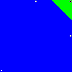
Regions classified by the SVM
The method cv::ml::SVM::predict is used to classify an input sample using a trained SVM. In this example we have used this method in order to color the space depending on the prediction done by the SVM. In other words, an image is traversed interpreting its pixels as points of the Cartesian plane. Each of the points is colored depending on the class predicted by the SVM; in green if it is the class with label 1 and in blue if it is the class with label -1.
Support vectors
We use here a couple of methods to obtain information about the support vectors. The method cv::ml::SVM::getSupportVectors obtain all of the support vectors. We have used this methods here to find the training examples that are support vectors and highlight them.
 1.8.7
1.8.7